Brownian Motion from Random Walks: A Mathematical Derivation Guide

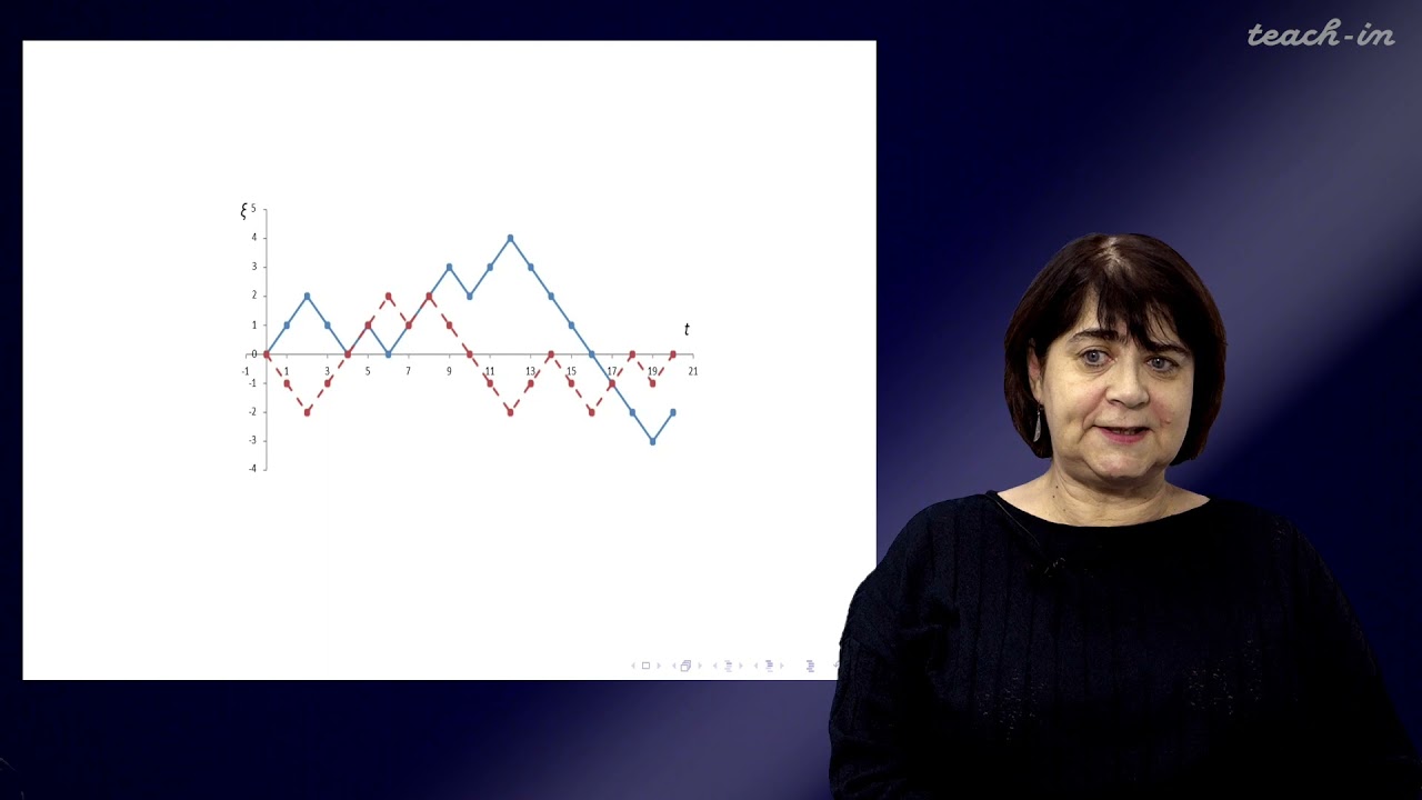
[00:00:00]hello so in this video we're going to try and build up a little bit of intuition behind where Brownian motion kind of comes from and such like so how are we going to do it how are we going to do it is by looking at what's known as symmetric what snows random walk now it's sometimes called the drunk-person walk because if you imagine you start at a point here you start at a point here and a sort of a drunk person is kind of walking around it goes to here then he goes here he goes to here and this is used to kind of model particles okay there's kind of you know you follow you move an even time step each time and effectively you end up with something which is fairly fairly random and obviously I'm not being random because I tend to you know it's impossible for a human being to be random because we're kind of programmed to do patterns and stuff but over time we basically end up with a with a random pattern okay so so basically just a drunk person walking around let's give it all that okay so this is what's known as a random walk and we're going to make it symmetric okay the way we should the reason why we're going to make it symmetric is because going to basically have a probability which is even okay so probability which is symmetric so probability or the half okay we're going to basically let the symmetric random walk we're going to knows it by the random variable xn okay and what we're going to basically do is we're going to start a process at zero so we're going to start like a counter if you like at zero okay and what we're going to look at is discrete time steps so basically what we're going to do is we're going to we're going to do something and we're going to cause a step and the value of the process either increases by one or decreases by one with the probability of 1/2 so we've got a probability of 1/2 and basically either go up by 1 or we go down by one with each time step okay so with each time step we either go up by why don't we go down what about the value which we're looking at now it goes up by one so the value of xn at each time step either goes up by one or down by one and what we can actually do is we going to toss a coin because the toss the coin is supposed to be random right supposed to be random okay it's got a probability of 1/2 and what we're going to basically do is we're going to toss a coin and for each toss of a coin if we get heads we're going to move up by one we're going to move the counter xn up by one but if we get tails we're going to go down by one okay so we're going to move the we're going to move xn down by one so effectively what we're doing if you want to kind of muddle it we've got xn okay and over time what we're going to do is build up we're going to build up value so we only going to go up by one or down by one now this is kind of the notation and we're going to go on from 1 to N okay and we're going to have a counter we're going to call it ZK okay so basically is better seeing it kind of by a graph okay we've got graph going on oh it could be negative as well okay could be negative and each time step kind of corresponds to a flick of a flip of the coin okay so we're going to start at 0 so this is xn going to start at 0 and let's say we get hits okay so maybe if I put in a little bit of an axis up here okay that's fine so you go 1 2 3 n Karen going minus 1 minus 2 and we start at 0 okay and this first time step the second time step this is third time step this is fourth time step this is fifth time step T equals one so sorry each time step is a flip of the coin since after the first flip the stuff for the second flip this after third fit full flip fifth let me carry on going basically we're going to do it for five flips and see what we value we end up with so I've got a coin here okay and I'm going to flip it you obviously can't see me flipping it I'm going to flip the coin okay so I flip the coin and we get tails now when we get tails we go down by one so we start at zero okay and we go down to negative one so you go down like that let me go flip it again okay I've got tails again so what we're going to do is we're going to go down by one again cases to the next time flip we're going to go down to one again to end up down here flip it again right we get heads so therefore we go up by one once we get up to here this isn't very well drawn obviously you you can draw it yourself better but there's a limit to what I can do it's flip it again heads again right go back up to here so we're back at zero and heads again okay so we're back up here now oops just get the time period okay so therefore this is kind of the this is kind of the random walk now of course we could have done it over and over again and we could have you know let's suppose let's do it again actually no no let's not do again you can do it again in your own time and you may have had sort of something which looks like this next time looks like that so we kind of go up and down a bit more but effectively you know this is this is kind of what we will be looking at okay so hopefully you're kind of building up this idea of a symmetric random walk okay now what I'm going to do not what we're going to do is we're going to start to toss the coin over smaller time intervals so let's say for example if I toss the coin once every once every once a second okay so that was tossing the coin once a seconds this is my time each second I'm tossing a coin okay now suppose I'm tossing the coin over a smaller time interval so I might for example get something that looks like this so he's like say for example over the time period of half a second say for example and let's use a blue plant over half a second okay so say get heads and the heart first half second then tails okay then perhaps I'll get heads again suppose I get heads again okay then suppose I get tails and heads again okay then the heads again and then let's suppose I get tails tails and then tails anyway something like that so basically we're tossing over a smaller time period so let's suppose to go there it's supposed to get there nastya pray to the end of kind of lost my bearings a little bit but yeah basically what I'm doing now is tossing over smaller and smaller time period now let's suppose I toss it again over another too late' smaller time period so suppose now I'd toss it over as another smaller time period they say a quarter of a second this time so I get something looks like this say okay so effectively what I'm doing is tossing over a smaller time period okay this is just kind of just missed that up anyway okay so a smaller time period again something looks like this I don't know I'm making this up now but yeah effectively hopefully you can see that what I'm getting is something that looks a little bit more Brownian motion like and then let's suppose I do it one more time okay but this time I do it over such a small time period that you can't see that kind of you you know you get it's basically looking like this so we get a small time period looks like this okay so small time period and basically you know this basically so basically every smaller and smaller time period I'm sort of going towards a kind of something looks like a Brownian motion so hopefully you can kind of see what I was doing with that example right so effectively you know it might discrete case so my discrete case in other words when I had when I had sort of definite time intervals you know one second or half a second or a quarter of a second in my discrete case I had what was known as a random walk I had what was known as a random walk okay so in my discrete case I had what was known as a random walk in other words I had two definite time steps then basically as I consider smaller and smaller time steps okay effectively my time interval was becoming smaller and smaller and smaller and effectively what I was doing is I was becoming continuous so in other words as my time steps becomes smaller and smaller and smaller so my time steps is going to zero okay I get what was known as a continuous case continuous case so instead of it being suddenly jerky movements it was now kind of as much smooth it becames much smoother rather than being kind of definite time intervals it became what was known as continuous in other words I didn't have to keep taking my time my paper my pen off the paper for each second right it became continuous and that's what was known as Brownian motion so in other words you know hopefully if you got the idea of random the random walk you know when I was tossing the coin I went up by one if I got heads and down by one if I got tails then based all I did is just considered a smaller and smaller time period smaller and smaller time period okay smaller and smaller smaller smaller smaller smaller okay until eventually I kind of became you know tiny tiny time and that's what was known as then Brownian motion so that's how random walks and Brownian motion are kind of connected to each other around the more correct Brownian motion respectively Brownian motion is just a random walk in a tiny tiny time steps tiny time steps okay okay so let's try and do a bit of maths with this now see what we've got okay so remember that we had our random variable xn which is for a symmetric random walk and we define that as the sum from k equals 1 to n of ZK right and let's just take ZK well remember we said the ZK was equal to one if you know at one if we had a hat if we had what was it heads we can it had a probability of 1/2 okay a negative one if it was a tails and again that also had a probability of 1/2 right well let's define ZK then if we divide our time interval into n equal steps okay so in other words we're kind of moving along here okay so we've got a random walk now okay kind of showing you how to derive the Brownian motion now let's try and look at some mathematical properties of Brownian motion so we have our random walk which is defined by which defined by xn equals the sum from k equals 1 to n of ZK and let's define you know let's divide like we did up here let's divide our time intervals to say it for example 5 we started off with 5 seconds and we defy you know we flipped a coin every second so therefore what we did effectively was divide our five second interval okay up into 5 into 5 equal time steps yeah because we tossed a coin every 5 time steps okay then what we did with every half a second what we were doing is again the same interval for 5 seconds but we're tossing every half a second so therefore we were defining of we're dividing our 5 second time interval up into 8 time intervals okay cause we're tossing one every half a second okay and then what we did with a quarter of a second same thing we had five second time interval but this time we're tossing every quarter of a second so it's we were dividing up into 60 yeah and then basically kept dividing up into smaller and smaller time steps in other words what we're doing what we're doing is we're dividing ZK up into T over N okay so we're dividing our time interval T which you have five seconds up into equal size time periods and the number of time piers that we had was n okay so for if we're tossing every second we're dividing up into flew n was five cases the Varia up into five equal time steps every half a second n was eight because we're dividing up into eight different time steps and so on and so and so on so as we got this now okay and what I'm actually going to do is for convenience I'm going to turn this into a square root okay and you'll see why I'm going to turn this into a square root in a minute and of course we can have the plus or minus root square root you can see where I'm going to have the square root in a minute because what I'm going to do is I'm going to try and find the expectation okay so what is the expectation of ZK what is the expectation of ZK well the expectation of Zed K would be zero okay because we've got a symmetric random walk so basically what we're asking is what would be the mean so we're starting at zero okay we're following some kind of random walks I'm kind of random pattern okay so what value would we expect to get out the end well we've got a problem in ax t of a half we've got a probability of the half so basically there's a half probability that we move up there's also a half probability that we move down okay so what would be the overall probability oops didn't mean to do that there we go what would what would what would be the overall probability what value would we expect said K to be what we'd expected to kind of stay the same because you know we either go up or we go down so therefore we kind of take the average of those two so you know we either go up so we only go to one or we go to minus one so the expectation is just the average of those two values so the value in the middle would just be 0 okay so the expectation should be 0 now what is the expectation of Z K squared what is the expectation of Z squared well it depends on how many installs were dividing up in twos we got our time interval it's going to be our time interval divided up into however however many steps that we divided up into isn't it okay so the expectation of Zed K squared should be T over m okay so therefore so basically if we if our expectation of Zed n is 0 then our expectation of xn okay which is just the sum of ZK so therefore if the sum of the if the expectation of ZK should be 0 okay if the expectation of said K should be 0 then X n which is equal to the sum of some of it said K should also be equal to 0 right because it's actually just like taking the sum of 0 right so it should be equal to 0 there's also an identity which I need to kind of which I need to kind of so basically what we can say is that those two things are equal to each other right because we've got xn is equal to that thing right right okay yeah right so there's an identity which I want to draw your attention to its EOF if we've got Zi and ZJ the expectation of two things multiplied together we can just break them up into the expectation of the first thing it's a linear operator right expectation of Z times the expectation of Z J okay and because they're kind of and they should both be equal to 0 because they're independent is that right or a con number anyway it yeah it's equal to 0 okay because the expectation of two things multiplied together should be 0 okay maybe onlys think about things because they're independent okay so let's have a look Lin what is the expectation of xn squared that's what we're after so we've got the expectation of xn is equal to 0 that's fine just by logic so what's the expectation of xn squared well the expectation of xn squared what's xn squared equal to what's xn squared equal to it is xn is going to be equal to well xn is going to be equal to xn is equal to the sum of ZK okay so xn is equal to the sum of ZK so therefore we would expect that it's the sum of Z K squared yes the sum of Z K squared so there was what we're saying is it's the expectation of Z 1 times you said 1 squared plus Z 2 squared plus wait a minute sorry that's not strictly correct as it because it's it's not the expectation of Zed K squared it's the expectation of all that squared because that's what xn is equal to so xn is equal to that so therefore X n squared should be that squared yes sorry that was my mistake so it's going to be z1 plus z2 plus right the way through to Zn right then okay and all of that squared all of that squared so effectively what we end up with is e of Z 1 plus a 2 plus a 3 2 Zn all right times same thing against Z 1 plus Z 2 plus right way through to wait - Zed n okay the expectation of all of that thing so let's just most play this thing out so we end up with well what's it going to look like so Zed one times ed ones that said 1 squared plus Z 1 times Z 2 right plus I'm just doing a Zed 1 versed - right the way through to said one time Zed n right and then we're going to carry on you can do the same thing now for Z - so it's Z 2 times ed 1 ok so Z 2 times Z 1 plus Z 2 times Z 2 so Z 2 squared right + right the way through to Z 2 times ed n okay plus right so look keep going so we got let's get rid of that please let me go ZN x ed what is it enzymes 8 1 + zip them n times Z 2 plus right the way through to Z 10 squared plus is it N squared okay now here's where we can make use of our identity here's where we can make use of identity because up here I've just said that the expectation of two things which are difference I and J so you know two things different said one say for example and said - or Zn and Zed one or whatever two things multiplied together can break up like this and it's going to be zero because the two things are going to be independent okay so it's going to be equal to zero so the expectation of two independent things are going to be equal to zero so there's what we can say is that those two things are different so they're going to go away they're going to be equal to zero okay those two things different they're going to be considered those two things different going to be equal to zero those two things different those two things are different those two things different so what we left with we're left with Z 1 squared we left with Z 2 squared and we're left with right way through 2 Z 10 squared so in other words what we're going to end up with is just the expectation of Z 1 squared plus said 2 squared right the way through to Z N squared so that was kind of what was writing first of all but I had to kind of take you through all the methods and stuff of where it came from rather right okay so therefore this is going to be equal to this is going to be equal to the expectation of Z 1 square cos it's a linear operator plus expectation of Z 2 squared plus right the way through to the expectation of Z 10 squared sorry was it N squared inside the brackets there we go and what have I set up here well I've said that the expectation of Zed's K squared is just going to be equal to T over N no matter what this K is is going to so whether it's 1 2 3 4 except to write went 3 whip 2 n it's just going to always be equal to T over N so therefore what do I end up with I end up with T over N so 80 over n plus T over N and that's T over N that's T over N right the way through to well that's T over N as well so they're all T over N so how many and how many T over N is do I have what I've got there's one two right the way through to n so we end up with n T over N to n times T over N the end is just cancel so I'm just left with T so in other words what I'm saying is the expectation of X N squared expectation of xn squared is just equal to T okay so in other words it's totally independent it's totally independent of time period it's totally independent of the number of number of steps that we have it doesn't matter there's no n over here there's no in on this right hand side set the expectation of xn squared no matter how many times steps that we take it's always going to be equal to T there's no end there okay so what do we have or for the discrete case discrete case of the case which we've worked out the very star the case of e of X n is equal to 0 and the expectation of xn squared is just equal to T okay then basically so this is this is kind of a random walk case then basically Brownian walk Brownian motion is when the number of time steps that we're taking or approaching infinity we considering smaller and smaller time steps in the same period okay in the same time period that we have the same time period you have to say from there to there this is time we just consider smaller and smaller time steps you can sit in more more time steps ok so the number of times since we have approaching infinity so because because these two things don't depend on the number of time steps that we take in other words we can say that with Brownian motion so in the continuous case continuous case okay oops that's supposed to say continuous continuous case what we basically end up with is exactly the same things it doesn't matter how many time steps we take because these two things here have don't have ends on the right hand side so in other words we can say that for Brownian motion for a random variable the expectation should be zero and the expectation of that random variable squared should be T okay so what does this mean well basically this as we approach infinity as we approach infinity as we approach infinity our random variable becomes Brownian motion this is now Brownian motion let's call it B I don't know let's call it B let's call it B T right likewise here we got B T so our experimental on the video we take more and more time steps okay we kind of become in continuous case which is Brownian motion okay so I've just shown you that as we take more time steps a discrete case becomes a continuous case we get exactly the same thing because the right-hand side doesn't pendel in okay so in other words we can say this about Brownian motion the expectation of Brownian motion is zero so in other words the expected value that we should get out of Brownian motion should be zero yeah which is kind of weird right and the expectation of Brownian motion squared should just be the time that it should just be whatever that time value at that time okay so basically what we can say now what we can say now is three properties okay so BT so the Brownian motion let's pull it Brownian motion at a time T so Brownian motion remains finite in other words because these two things don't tend off don't shoot off to infinity basic what we say is they remain bounded or they remain finite it's a Brownian motion should remain within a given kind of title should remain within some certain finite interval okay also we can say two things which we're going to talk about later on in the course anyway but I can talk very briefly about them now Brownian motion is a Markov process a Markov process and it's also a martingale okay so a Markov process is kind of is kind of just saying that what you know these two think there's these two things let's try to put them into perspective of all kind of financial derivatives in minute but effectively Markov process and Markov process is just memoryless so in other words it doesn't matter what comes before okay it's kind of forgetting it's a bit like goldfish Markov is just a goldfish right it's only got five second memory it can't really remember what happens before that time okay so it's a memoryless process Brownian motion like I was saying you know before right you know in the previous video Brownian motion it has independent time periods or time increments so in other words what that means what that means is that that time period is totally independent of all other time piers that have come before it it doesn't matter what's happened before it doesn't matter about the past yeah it's just what happens at that point in time now so that's what a Markov process space is describing now a martingale is a lil is a little bit different it's a little bit different Brownian motion remaining finite let's just talk about that in terms of them in terms of you know a financial point of view well this is basically saying that it cannot carry on forever the Brownian motion cannot carry on forever it's a brown bounded process okay so in other words what that means is that the share price which can be described using a Brownian motions share price of something cannot go zooming off to infinity so basically as a company cannot have an infinite amount of work it will always have a finite amount of work so that's what this kind of means it cannot have an infinite amount of an infinite amount of worth it cannot have that okay Tanel it cannot have an infinite amount of worth okay the Markov process basically saying is memoryless so whatever happens in the path it doesn't matter the past the past as far as the Brownian motion is concerned it doesn't matter it's just what happens at that point in time now martingale this is a little bit different basically the idea is is that the best guess for what's happening for what's going to kind of happen next is what's happening now okay so the best guess with what's happening let me write this down the best guess but what's kind of future so the future if you like so the best guess for the future is what's happening at this time point now in other words it's not going to change this is what a mark this is what a martingale is okay effectively it's basically saying that what's going to happen in the future is the same as what's going to happen now that's the best guess that you can make okay so it's expectedly the same as you've got stay so for example if you've got twenty dollars in your company today if your company's kind of if your share price is worth twenty dollars today okay then that basically means that it may also be worth twenty dollars tomorrow and we worth twenty dollars the day after that and the twenty dollars the day after that so basically what this is saying is that your share price is always going to say at twenty dollars is always going to say at twenty swords now of course we know it doesn't okay but it's kind of a paradox because what we're basically saying is that we're not going to make any money on our share price we've got a share price as well $20 with a basic saying is going to stay at $20 so we're not going to make any money but in actual fact we can exploit that fact to make money it's kind of a little bit of a paradox okay we're basically saying that you know we're not going to make any money but we can use that fact to make money the reason why the reason why that's important the reason why that's important is because the share price today contains all the information about the past so the share price at this moment in time so say if we have a number line okay the share price at this moment in time today may be four right over here actually this is the time period we're at this point in time so the share price at this point in time contains all the information about the past okay so if we try and kind of look at this and try and predict some kind of pattern based on what's happened in the past I mean of course this is why we use the martingale process the Markov process that it's a memoryless process but basically if we try and look at the past try and spot a pattern then act on that pattern then the very act then the very act of kind of looking at the pattern trying to kind of act on that pattern will change the future pattern so in other words if you like it's got you know it's got a set path you know the share price is say following something like this okay and you know save with this point in time here and we kind of it should carry on like this it knows which path is going to carry on say for example it's going to carry on in this path but basically we're going to look at what's happened in the past and we're going to try and predict that it's going to happen on this path well our actions are predicting what's going to happen on the past is actually going to change the share price so other words we've got something looks like this okay and it should carry on like this okay but because we can kind of look at the past and we can kind try and spot some pattern then we kind of try and act on that to try and exploit as much money as possible based on the predicted pattern okay but that action of acting on it say for example would go out and buy more shares right will affect what's going to happen in the future buying more shares will obviously affect you know other things elsewhere so affects what we're going to end up with is we're going to actually our action is actually going to change what the patterns going to look like for example maybe that's a bad thing one final thing about Brownian motion is that of course if we look back up here if we look back up here okay it's going to become kind of like something like this and it's what's known as a fractal okay so it's going to become something like this as we consider small and smaller time steps it's going to become more and more random going to go more like this and this kind of this kind of shape and it's known as a fractal so basically we do is we zoom in on a section of the graph we zoom in on the section of the graph and it's still looking like this then we zoom in on this section of the graph say excuse me and it looks like this okay so in other words no matter how many times we zoom in we still get this jagged up you still get this jacket pattern where as with most graphs if it looks say something like this you know if we zoom in effectively as soon as we start zooming in we expect it to kind of become smoother okay until affectionally we come a straight line okay so what that's one of the biggest difficulties that basically you know this kind of theory with most functions in that basically be zoom in far enough it becomes a straight line we can then use that to differentiate and find out what the rate of changes but because most share prices follow a Brownian motion and when we zoom in we still get jagged patterns so in other words it doesn't approach a straight line we can't use standard differentiation techniques we actually have to use something called stochastic differentiation which involves probability as well okay but we'll come to that in future videos