





![[Fall-2022] Tutorial: Probability](https://i.ytimg.com/vi_webp/rcXeRCGCh4o/maxresdefault.webp)











![The Feynman-Kac formula, partial differential equations and Brownian motion [QCT21/22, Seminar #12]](https://i.ytimg.com/vi/oXaUfqdQyas/maxresdefault.jpg)

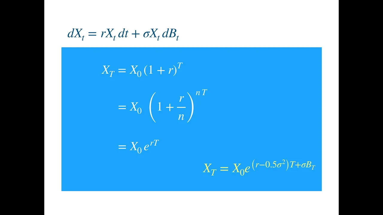
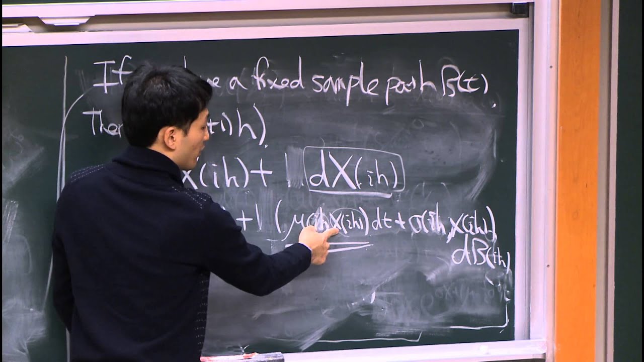
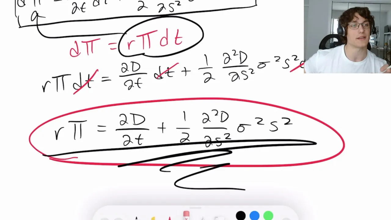
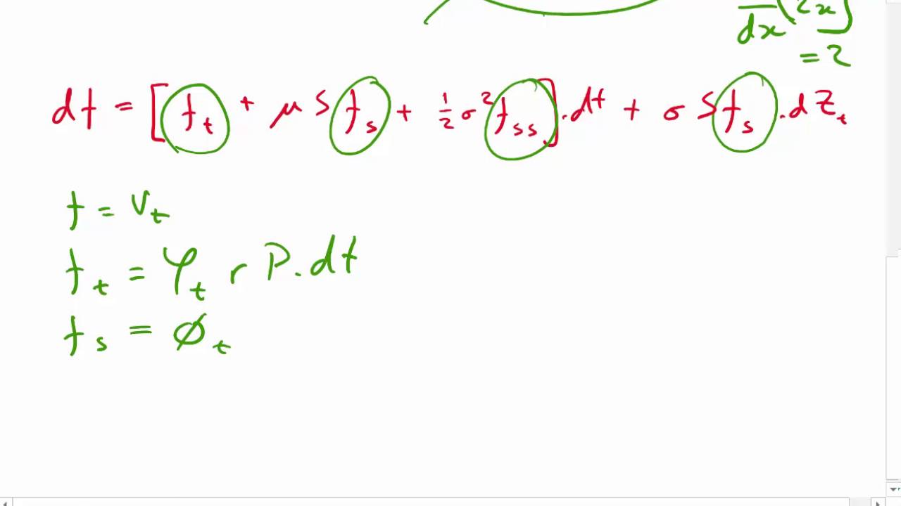
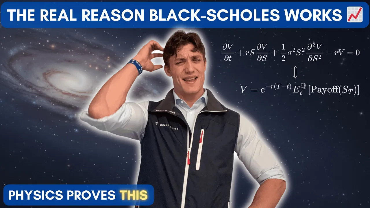
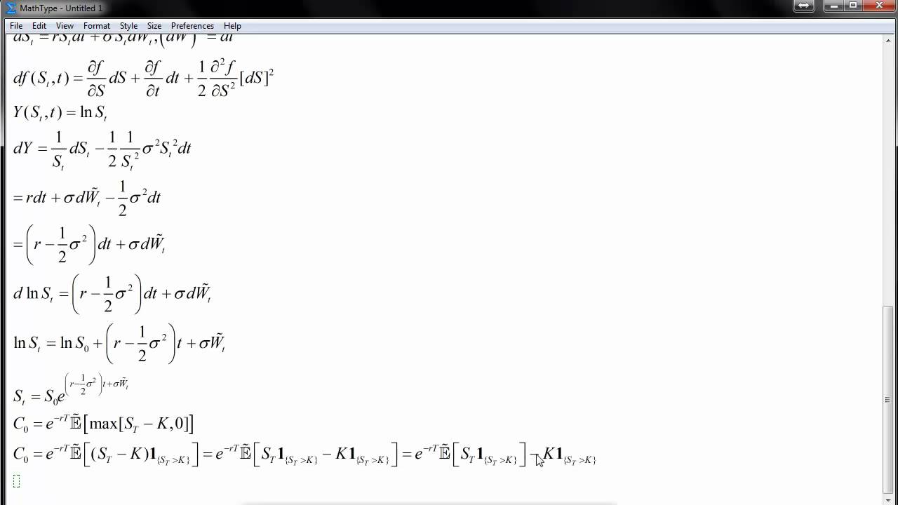
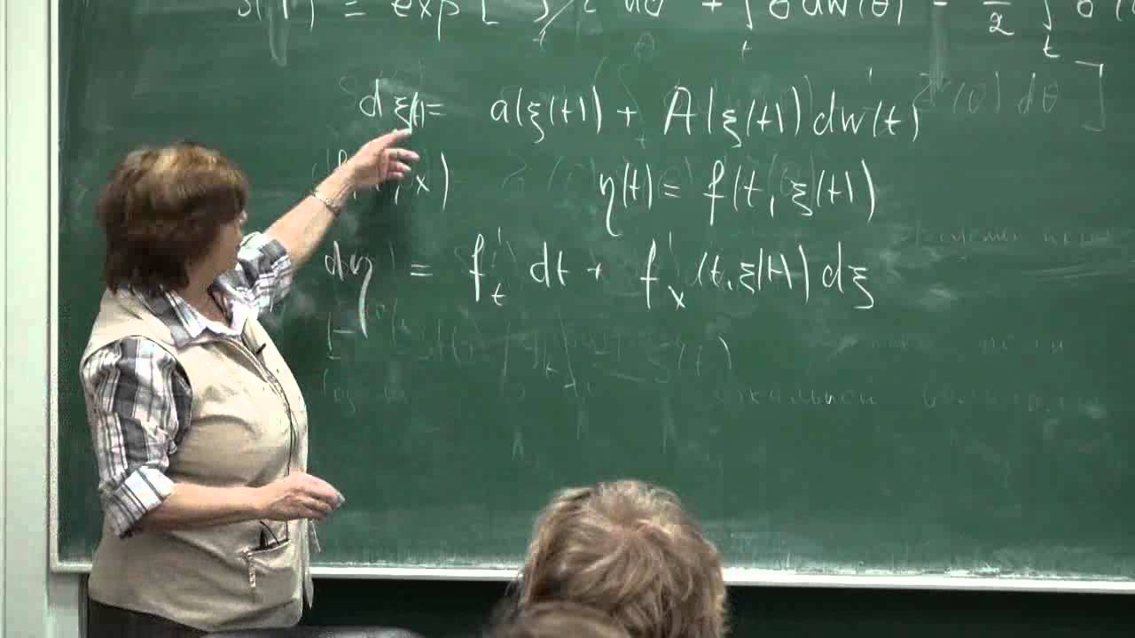
Itô calculus extends classical calculus to handle stochastic processes by incorporating quadratic variation, which for Brownian motion equals the time interval. The key insight is that when applying Taylor expansion to functions of stochastic processes, the second-order term involving dB² survives because dB² = dt, unlike classical calculus where such terms vanish. This leads to Itô's lemma: for a function f(t, X_t) where dX_t = μ(t,X_t)dt + σ(t,X_t)dB_t, the differential is df = [∂f/∂t + μ∂f/∂x + (1/2)σ²∂²f/∂x²]dt + σ∂f/∂x dB_t. The additional (1/2)σ²∂²f/∂x² term distinguishes stochastic from classical calculus. This framework enables modeling financial instruments like geometric Brownian motion for stock prices, where the drift adjustment (1/2)σ² ensures the process has no natural tendency to rise or fall, making it a martingale under the risk-neutral measure.
Itô Calculus Explained: Brownian Motion and Stochastic Integration
Added:the following content is provided under a Creative Commons license your support will help MIT open courseware continue to offer highquality educational resources for free to make a donation or view additional materials from hundreds of MIT courses visit MIT opencourseware at ocw.mit.edu so let's begin today we're going to continue the discussion on EO calculus so I briefly introduced you too LMA last time but let's begin by reviewing it and yeah stating in a slightly more general form okay so last time what we did was we did quadratic variation of brownan motion brownan process or I call it brownan process we defined the Brownian process Brownian motion and then show that it has quadratic variation which can be written in this form DB s is equal to DT and then we use that to show the simple form of EOS LMA which says that if f is a function on the Brum motion then D of f is equal to F Prime of DBT plus F Prime of DT so this additional term was a characteristic of EO calculus In classical calculus we only have this term but we have this additional term and if you remember this happened because exactly because of this quadratic variation so let's review it I mean let's do it in a slightly more general form so assume now we have a function f depending on two variables T and x and we're interested in we want to evaluate our high of information on the function ft BT okay the second coordinate we want to we're planning to put in the Brownian motion there then again let's do the same analysis can we describe D of f in terms of the differentiations so to do that okay just like this let me start from tailor expansion so F at a point t plus delta T X+ Delta X by Tailor expansion for two variables is f of T of X Plus F DF partial partial of f over partial of T at T comma X of delta T plus X okay that's the first order terms and then we have the second order terms and then the third order of terms and so on so that's just tailor expansion if you look at it we have a function f we want to look at the difference of f when we change the first variable a little bit and the second variable a little bit so it start from F of T of X in the first order terms you take the partial derivatives so take d f over d t and then multiply by the T difference second term you take the partial derivative with respect to the second variable partial F over partial X and then multiply d x that much is enough for classical calculus but then as we have seen before we want to look at the second order term so let's write first write down what it is that's exactly what happened in Taylor expansion if you remember if you don't remember just believe me this one over two * takes the second part second derivative partial okay so let's write it in terms of yes should oh yeah you're right you yes is it good now yeah okay so let's write it as DT all this [Applause] Deltas just write like that I'll just not write down t of X and what we have is f+ d f over DT DT d f/ d x DX plus the second order terms okay so the only important terms first of all these terms are important but then if you want to use xals B of T So if you're now interested in f t comma B of t or more generally if you were interested in Ft + DT F VT + D of VT then these terms are important so if you subtract F of T of VT which you get as these two terms just Del F over d t DT plus d f over DX I'm just writing this as a second second variable differentiation at DBT and then the second order terms instead of writing it all down DT sare is insignificant and DT DT * DBT also is insignificant but the only one thing that matters will be this one this is DBT Square which we saw is equal to DT so from the second order term you'll have this term surviving 1/ two partial F over partial X second derivative of DT that's it okay if you rearrange it what we get is partial F over partial t plus half this and that's the additional term if you ask me why these terms are not important and uh these terms are not important and these term this term is important well I can't really say it rigorously but if you think about DBT s = DT D * BT is kind of like square of DT it's not a good notation but if you use that these two terms are significantly smaller than DT because you're taking a power of it DT s becomes a lot smaller than DT DT the 32 is a lot smaller than DT and but this one survives because it's equal to DP here that's just a high level description okay that's a slightly more sophisticated for form of EOS LMA let me write it down here and let's just fix it now f is T of BT then uh that's D of f is equal to any questions just remember from the classical calculus term we're only adding this one term there yes why do we have X is uh just to because the second variable is supposed to be X and then I don't want to write down partial derivative with respect to a Brownian motion here because doesn't look good so it just means take the partial derivative with respect to the second term so just view this as a function f of T of X evaluate it and then plug in xal BT in the end yeah yeah because I don't want to write down partial BT here other questions okay this now this uh consider stochastic process X of t such that D of X is equal to Mu * D of t plus Sigma * T of PT okay so this is almost like a Brownian motion but you have this additional term this is called a drift term and basically this happens if XT is equal to Mt plus Sigma VT if mu and sigma are constants from now on what we're going to study is stochastic processes of these this type whose difference can be written in terms of some time U drift term and the Brum motion term so we want to do a slightly more general form LMA where we want F of T of XT here that will be the main object of study I'll finally State the strongest EOS Lima that we're going to use f is some smooth function and XT is a stochastic process like that XT satisfies where BT is a Brum motion then DF of txt can be expressed as okay it's just getting more and more complicated but it's based on this one simple principle really it all happens because of the quadratic radiation I'll will show you why this form it Devi this form deviates from this form when we replace B to an X okay so remember here all other terms didn't matter but the only term that mattered was partial square of f of Delta x² DX s okay so to prove this note that DF is partial F over partial T DT plus partial F over partial x d of XT plus half of D of x^ 2 just exactly the same but I repl the DB previously what we had DB I'm replacing to DX okay now what changes is DX can be written like that if you just plug it in what you get here is yes uh partial F or partial X MDT plus Sigma of DBT now what you get here is 12 of partials and then mu DT plus Sigma DBT s out of the three terms here that we get mu s DT square + 2 * mu Sigma D mu db+ Sigma squ DB Square only this one survives just as before these ones disappear and then you just collect the terms so DT there's one DT here there's mu * that here and that one will become a DT so it's half of Sigma squ s DT and there's only one DBT term here Sigma and I made a mistake yes okay so this will be the form that you'll use it the most because you want to evaluate some stochastic process a difference uh some function that depends on time and that stochastic process you want to understand the difference DF and then DX will the X would have written in terms of a browni motion and a drift term and then that's it toal for it okay so but if you want to just if you just see this for the first time it just looks complicated too complicated you don't understand where all the terms are coming from but in reality what it's really doing is just take this tailor expansion remember these two classical terms and remember that there's one more term here you can derive it if you want to oh really try to know where it all comes from it all started from this one fact quadratic variation because that made some of the second derivatives survive and because of those we get these kind of complicated terms questions okay great let's see some examples that's too much of a there's too much sorry I'm going to use it a lot so let me record it example number one let F ofx be equal to x² okay and then want to compute D of f f BT I'll give you like three minutes just to try practice you manage to do this okay so it's a very simple example yes okay so assume it's just a function of two variables but it doesn't depend on T well you don't have to do that but let me just do that and partial over partial F over partial t0 partial F over partial X is equal to 2X and the second derivative equal to two at TX so now we plug in t comma BT yeah and yeah what you have is mual 0 Sigma = 1 if you want to write it in this formula okay so what you're going to have is 2 * BT of DBT + 1 / 2 * 2 D right them you can either use these parameters and just find that just plug in each of them to figure it out or a different way to do it is really write down remember the proof this is partial F over partial T DT plus partial F over partial X DX + 12 remember this one and next is the BT here that one is zero that one was 2x so 2bt DBT and you do it one more time so you get DT cool make sense okay let's do few more examples yeah just one more second one is this that one and you want to compute D of F at T comma B of T so maybe I'll just do it this time so again partial F over partial T DT plus partial F over partial X DBT that's the first order terms the second order term is 12 partial Square F partial x² of DBT s which is equal to DT and let's do it partial F over partial T you get mu * F this one is just equal to Mu * F or maybe I'm going too quick is Mu * e mu t + DX DT partial F over partial X is Sigma * mu t + DX and then DBT plus if you take the second derivative you do that again what you get is 12 and then Sigma squ * e to Mt + DX DT yes and the original equation that you just wrote is it Sig and then the second here yesare oh Sigma okay that's a good question but that Sigma is different that's if you plug in XT here if you plug in an XT where XT is equal to Mu Prime DT plus Sigma Prime D of BT then that Sigma Prime will be become a sigma Prime Square here but here the function is Mu and sigma but so maybe it's not a good notation let me use a and b here instead the sigma here is a different from it's different from here yeah if you replace a and b then these are yeah but I already wrote down all M that's a good point actually so but that's when you want to consider a general stochastic process this here other there than branium motion but here it's just a Brum motion so it's the most simple form and that's what you get and this is what you get it's mu + half Sigma squ and these are just all F itself that's a good thing about exponential f * DT plus Sigma * D of BT okay make sense okay and there's a reason I covering this example it's because let's come back to this question you want to model stock price stock price using Brownian motion Brownian process s of T but you don't want St to be a Brum motion what you want is a difference percent percentile difference to be a Brownian motion so you want this percentile difference to behave like a Brownian motion with some variance okay the question was is stal to e to the sigma * B of T in this case and I already told you last time that it's no it's not true and we can now see why it's not true so take this function stal e to Sigma BT that's exactly when mu is equal to zero here what we got here was D of St in this case is equal to Mu is 0 so we get 12 of Sigma squ * DT plus Sigma * D of BT we originally was were targeting at Sigma * DBT but we got this additional term which we didn't want in the first hand in other words we have this drift okay I haven't I wasn't really clear in the beginning but our goal was to model stock price where the expected value is zero at all time so our guess was to take e to Sigma BT but what turns out that in this case we have a drift if you just take naturally e to Sigma BT so to remove that drift what you can do is subtract that term somehow if you can get rid of that term and you can see if you add this to be minus 1 2 Sigma squ you can remove that term okay that's why it doesn't work so instead use what is it s of t = e to the - 1 / 2 Sigma s uh t plus Sigma of B so that's a geometric brownia motion without drift and the reason it has no drift is because of that if you actually do the computation the DT term disappears okay question okay so far we have been discussing differentiation now let's talk about integration yes could you just I mean so we do get this solution as of MH you also describe what it means so what does it mean this this solution this solution B yes yes so does that mean if we have a sample p BT then we could get the sampi for oh what this means yes so when whenever you have the BT values just at each time takes exponential value because we why we want to express this in term of brownie emotion is for Brownian motion we have a very good pretty good understanding it's a really good process you understand fairly well and you can you have good control on it but the problem is you want to have a process who percentile difference behave like a Brum motion and this gives you a way of describing it in terms of Brownian motion as exponential function of it so and is that does that answer your question or right yes so this equation means that if we have a sample path BT M that would give a corresponding sample P for is it like a point wise evaluation oh that's a good question actually but yeah think of it as a point where evaluation that is not always correct but for most of the things that we will cover that's it's safe to think about it that way yeah but if you think about it paf all the time eventually it fails but that's a very Advanced topic so so what this question is is basically BT is a probability space it's a probability distribution over passes so this equation just look at it it looks right but doesn't really Mak sense because BT if it's a probability distribution what is e to a BT okay well basically what it's saying is BT is a probability distribution over passes so if you take omega according to a pass according to the browni motion sample uh probability distribution and for this path it's well defined this function okay so the probability dens density probability density function of this path is equal to the probability density function of e to the whatever that is in this distribution okay maybe it confused you more just consider this as some path has some well- defined function and you have a well defined function okay so what was I trying to do oh integral definition I will first give you a very very stupid definition of integration we say that uh we Define f as an integration okay if D of FAL to F DT it's just we Define it as an inverse of differentiation because differentiation is now all defined we could we just Define integration as the inverse of it just as in what is it classical calculus so so far it doesn't have that good meaning other than being an inverse of it but at least it's well defined the question is does it exist I mean does it given f and g does it exist does integration always exist and so one there's lots of questions to ask but at least this is some definition and the natural question is does there exists a remanion some type description that means if you remember how you define integral in calculus [Applause] don't you have a function f a very good function f the integration of f from A to B according to the remion some distri description was you just chop the interval into very fine pieces A1 a0 A1 A2 A3 dot dot dot and then sum the area of these boxes and takes a limit so this was a limit of ranan sums okay slightly more if you want is it's the limit as n goes to Infinity the function 1 n * sum of I 1 to T I'll just call Z to b f of TB / nus f of tus1 that bring bring up L okay but question no you're right good point no we don't yeah thanks so does inter inte inter integral defined in this way have this remion some type description the question so keep that in mind I will come back to this point later and in fact it's a very deep it turns out to be a very deep question and very important question this question because if you remember like I hope you remember in the ranian sum it didn't matter which point you took in this interval okay that was the whole point you have the function in the interval AI to AI + 1 you take any point in the middle and make a rectangle according to that point and then no matter which point you take when you go to the Limit you had exactly the same sum all the time that's how you define the limit but really interestingly like what's really interesting here is that it's not no it's no longer true if you take the left Point all the time and you take the right Point all the time the two limits are different and again that's due to the quadratic variation because that much of variance can accumulate over time okay so that's the reason we didn't start with a reming sum type definition of integral but I'll just make one remark e to integral is the limit of ranan sums when always take the leftmost point of each interval okay so you chop down this curve at the time interval into pieces and for each rectangle pick the left move point and use it as a rectangle okay and you take the limit that will be your EO integral defined it will be exactly equal to this thing the inverse of our to differentiation I won't be able to go into detail what's more interesting is instead what happens if you take the rightmost point all the time you get an equivalent theory of calculus so it's just like eo's calculus it looks really really similar and it's coherent itself so there's no logical flaw in it it all makes sense but the only difference is instead of a plus in the second order term you get minuses yeah so let me just make it as a remark but because I it's just a theoretical part thing but I think it's really cool so we Mark there exists an equivalent version maybe equivalent is not a right word but a very similar version of EO calculus such that basically what it says is DBT s is equal to minus DT then that changed a lot of things but this far just it's not that important it's just a fun like cool stuff so let's think about this a little bit more this fact taking the leftmost point all the time means if you want want to make a decision for your time interval so at time T of I and time T of I + 1 let's say it's a stock price you want to say that you had like so many stocks in this time interval let's say you had so many stocks in times this time interval according to the values between this and this in real world your only choice you have is you have to make the decision at time T ofi your choice cannot depend on the future time you can't suddenly say okay in this interval my the stock price increased a lot so I'll assume that I had a lot of stops in this interval okay in this interval uh it I knew it was going to drop so I just going to take the rightmost interval like I'm going to take I I'll assume that I only had this many stuff you can't do that your decision has to be based on the leftmost point because the time you can't see the future and the reason EOS calculus is so works well in our setting is because of this fact because it has inside it the fact that you cannot see the future every decision is made made on the leftmost time so if you want to make a decision for your time interval you have to do it in the beginning that intuition is like hidden inside of the theory and that's why it works so well now let me iterate that part a little this part a little bit more there the definition of these things where you're only allowed to at up at time T you're only allowed to use the information up to time T and there is I should have it so definition delta T is an adapted process sorry uh ad that is adapted to another castic process XT if for all values of time variables delta T depends only on x0 up to XT there's a lot of vague statements inside here but what I'm trying to say is just assume X is a Brownian motion underlying stock price so your stock is changing you want to come up with a strategy and you want to say that mathematically the strategy makes sense and what it's saying is if your strategy makes your decision at time T is only based on the past values of your stock price then that's an adapted process so this defines the processes that are reasonable that cannot future and these are in terms of strategy if delta T is a portfolio strategy these are the only meaningful strategies that you can use okay and because of what I said before because we're always taking the leftmost point this adapted processes just also fit very well with EOS calculus all comes into play alog together just a few examples so first a very stupid example XT is adapted to XT of course because at time T XT really depends only on XT nothing else two XT + 1 is not adapted XT well this is maybe a little bit fague so call YT = x t + 1 YT is the value at t + 1 and it's not based on the values of to time T just a very artificial example but another example can be uh Delta tals minimum is adapted and I'll let you think about it the force is quite interesting suppose T is fixed some large integer or some large real number then you let delta T to be the maximum of X of T delta T yeah where S Sub s where T is from okay it's not adapted what is this this means at time T I'm going to take at it this value a maximum the maximum of all values inside this part the future so this refers to the Future it's not an adapted process any questions okay so now we're ready to talk about the properties of Ito ito's integral just let's quickly review what we have first divined uh first I defined EO LMA so that means differentiation in EO calculus then I defined integration using differentiation integration was an inverse operation of the differentiation but this integration also had an alternative description in terms of remanion sums where you're taking just the leftmost interval leftmost point at as the reference point for each interval and then as you see this naturally has this concept of using the leftmost point and to abstract that concept we come up with this adapted process very natural process which is like the real life procedures Real Life Strategies we can think of now let's see what happens when you take the integral of adapted processes each integral has really really cool properties okay okay so the first thing is about normal distribution BT has normal distribution 0 to T so your Brum motion at time T has normal distribution with 0 t that means if your stochastic process is some constant time V of T of course then we have 0 and c² T still normal variable that means if you integrate that's the integration of some Sigma yeah yeah that's the integration of Sigma DBT so if Sigma is a fixed constant when you when you take the to e to integral of DBT Sigma time DBT this constant at each time you get a normal distribution and this is like saying the sum of normal distribution is also normal distribution it has this hidden fact because integral is like sum in the limit and this can be generalized so if delta T is a process depending only on the time variable so it does not depend on the Brum motion then the process X of T equals the integration of delta T DBT has normal distribution at all time just like this we don't know the exact variance yet the variance will depend on the sigmas but still it's like a sum of normal variables so we'll have normal distribution that's one fact and it just gets better and better a second fact is called EO isometry okay that was cool can we compute the variance [Applause] EXC yes can you that board off yeah sure does it go up oh this one doesn't go up that's a bad yeah so I'll do it later I wish this do go [Applause] up okay so this has a name called e to isometry can be used to compute the variance so BT is a Brownian motion delta T is adapted to a Brownian motion which is brown your motion then the expectation of your E2 integral that's the E2 integral of your redaptive process that's a variance so you take the square of it is equal to something cool your Square just comes in quite nice isn't it before I won't prove it but let me tell you why just we already saw this phenomena before this is basically quadratic variation and the proof also uses it if you take Delta s equals to one sorry I was using Korean one at all time then what we have is here you get a Brum motion BT so on the left you get like expectation of BT square and on the right what you get is like T because when Delta s is equal to one at all time when you integrate from 0 to t you get T and you have t on the right hand side that's what it's saying and that was the content of quadratic variation if you remember we were summing the squares maybe not exactly this but you're summing the squares over small intervals okay yeah that's some really good fact that you can use to compute the variance right you have an A2 integral you know the square can be computed just in this simple way that's really cool okay and one more property this one will be really important you will see it a lot in future lectures is that when is e integral of Martingale what was a Martingale Martingale meant if you have a stochastic process at any time T whatever happens after that the expected value at time T is equal to zero okay so it it doesn't have any natural tendency to go up or go down no matter which point you stop your process and you see your future it doesn't have a natural tendency to go up or go down in uh formal language it can be defined as where ft is the events x0 up to XT so if you take the expected conditional expectation based on whatever happened up to time T that expectation will just be whatever value you have at that time intuitively that just means you don't have any natural tendency to go up or go down question is when is or each to integral I'm marting okay adapted to B of T then it's a mar as long as G is not some crazy function as long as G is reasonable one way you can be reasonable if it's L2 Norm is bounded if you don't know what it means just you can safely ignore it basically if G doesn't like it's not a crazy function if it doesn't grow too fast then in most cases this integral is always a marting okay so if you flip it remember integral was defined as the inverse fun inverse of differentiation so if dxt is equal to some function mu that depends on both T and BT * DT plus Sigma of DBT what this means is XT is a marting gale if that is zero at all time always okay and if it's not zero you have a drift so it's not not a marting gale okay Z that gives you some classification now if you look at a differential equation of this stochastic this is called a stochastic differential equation if you have a stochastic process if you look at a stas differential equation if it doesn't have a drift term it's a marting gale if it has a drift term it's not a marting gale that will be really useful later so try to remember it the whole point is when you write down a stochastic process in terms of something times DT something time DBT really this term contributes towards the what is it tendency like the slope of whatever is going to happen in the future and this is like the variance term it just it adds some variance to your stochastic process but still it doesn't add add our subtract value over time it's really fair Fairly like yeah fairly adds variation remember that that's very important fact you're going to use it a lot for example you're going to use it for pricing theory in pricing Theory you come up with this stochastic process or some strategy you look at its value like let's see XT is your value of your portfolio over time if that portfolio has yeah then you match it with your financial what it let me go over slowly again first you have like a financial derivative like option of a stock and then you have a portfolio strategy assume that you have some strategy that at the expiration time gives you the exact value of the option now you look at the difference between these two stochastic processes basically what it's saying is when your variance goes to zero your drift T has to goes to zero so when you look at the difference if you can somehow get rid of this variance term that means no matter what you do that will govern the value of your portfolio if it's positive that means you can always make money because there's no variance without variance you make money that's called Arbitrage and you cannot have that B that but yeah I won't go into further detail because facil will cover it next time but just remember that flavor so when you write something down in a stochastic differential equation form that term is a drift term that term is a variance term and if you don't have drift it's a markting gale that is very important any questions that kind of the basics of it calculus I will give you some exercises on it mostly just basic computation exercises so that you'll get familiar with it try to practice it and let me cover one more thing called Cen of theorem it's related but yeah these are really basics of the toal so if you have any questions on this please ask me right now before I move on to the next topic Okay so the last thing I want to talk about today [Applause] here is a underlying question suppose you have two Brum motions this is without drift and you have another B Tilda Brum motion with drift so it's just some prob these are two probability distributions over passes according to BT you're more likely to have M branium motion that has no drift that's what let's say that's what sample path according to B Tilda you have some drift and around your motion move close move closer CL okay so typical path it will follow this line and we'll follow that line and the question is this can we switch from this distribution to this distribution by a change of measure can we switch between the two measures to probability distributions by a change of measure let me go a little bit more what it really means so assume that you're just looking at a brown your motion from Time Zero up to time T some fixed time interval then according to BT let's say this is path a sample path Omega you have some probability of Omega uh this is a PDF given by this Brownian motion B and then you have another PDF P Tilda of Omega where the PDF given by of T the question is does there exist a z depending on Omega such that P of Omega is equal to Z * p okay do you understand the question okay clearly if you just look at it they're quite different the passes that you get according to distributions are quite different it's not clear why why should we should expect it at [Applause] all and you'll see the answer soon but let me discuss what all this in the Contex different context just forget about all the brownie motion and everything just for a moment and this concept changing from one probability distrib dist to another distribution it's a very important Concept in analysis and probability just in general theoretically and there is a name for this Z for this changing measure if Z exists it's called the radon nikodim Ron nikodim derivative so let me before doing that let me talk a little bit more okay so suppose p is a probability distribution over Omega it's a probability distribution so this is some set and P describes the probability that you have each element in the set and and you have another probability dist plda another probility distribution so we Define p and p Tilda to be equivalent if the probability that a is greater than zero if and Only If For All these probability distributions describe the probability of the subsets so let me let's just think about a very simple case Sigma is equal to 1 2 and 3 P gives 1/3 probability to 1 1/3 probability 2 1/3 probability to 3 p Tilda gives 23 probabilities to 3 1/ six probability to 2 1/ 6 probability to three so we have two probability distribution over some space they are equivalent if whenever you take a subset of your ground set let's say 1 two when a is equal to 1 2 according to probability distribution P the probability you have you fall into the set a is equal to 2/3 according to P Tilda you have 56 they're not the same the probability itself is not the same but this condition is satisfied when it's zero is when it's not zero is not zero and you can just check that it's always true because they're all positive probabilities on the other hand if you take instead say 1/3 and zero now you take your a to be three then you have 1/3 equal to zero so this means according to probability dist distribution P there is some probability that you'll get three but according to probability distribution P Tilda you don't have any probability of getting three so they're not equivalent in this case if you think about it then it's really clear so the theorem says this is a very important theorem analysis actually the theorem there exists a z such that uh P of Mega is equal to if and only if p and p Tia are equivalent you can change from run one probability measure to another probability to meas measure just in terms of multiplications if and only if they're equivalent and you can see that it's not the case for this when they're not equivalent you can't make a zero probability to 1/3 probability by multiplication so in the finite world this is very just intuitive theorem but this what this saying is is true for all probability spaces and the is called the ronm derivative our question is are these two Brownian motions equivalent the paes that this Brownian motion without drift takes and the Brownian motion with drift takes are they kind of the same but just skewed in distribution or are they really fundamentally different that's the question okay and what gers of theorem says is that they are equivalent Al to me it came as a little bit not inuitive I would I would imagine that it's not equivalent these two just like these paths have a very natural tendency as you go to Infinity these PS and these pests will really look a lot different because when you go really really far the passes which have drift will be just really close to your line mu of t while the pathes which don't have drift will be really close to the x-axis but still they are equivalent you can change from one to another I'll just state that theorem without proof and this will also be used in pricing Theory and I can't really tell like I'm not an expert enough to tell why but basically what it's saying is you switch some stochastic process into a stochastic process without drift that's making it into a marting gale and Martingale has a lot of meaning in pricing Theory as you will see so this also has application that's why I'm trying to cover it Al it's quite a technical theorem try to remember at least this statement and the spirit what it means it just means these two are equivalent you can change from one to another by a multiplicative function okay a good place to ra okay let me just state it in the simple form jle interject yeah sure with um these uh sort of changes of measure it it it turns out that um all of these theories uh with continuous time processes should have an interpretation if you discretize time and sort of consider sort of a finer and finer discretization of the process and um with this change of measure um if you consider problems in discreet uh stochastic processes like uh random walks you know basically how uh say if you're gambling against you know uh a casino or against another player and you look at how you're winnings evolve you know as a random walk depending on your odds your odds could be that you will tend to lose so there's basically a drift in your wealth as as this random process evolves you can transform that process to a pro basically by taking out your expected losses to a process which has sort of zero or change in expectation and so you can convert sort of these uh gambling problems where there's drift to uh a version where there's G where where the process essentially has no drift and it's a Martingale and the Martingale theory in stochastic process courses is very very powerful there's Martingale convergence theorems so you know that sort of the limit of the Martingale is uh basically there's convergence of the process and and that applies here as well so do you will see some surprising applications yeah and so try to at least digest is a statement because when the guest speaker comes and says by gers of theum you actually actually know what it is in the spirit okay so Cur enough this is a very simple version there's a lot complicated versions but let me just state it okay so p is a probability distribution over passes from OT to Infinity what this means is just passes from uh that stochastic process defined from Time Zero up to time T so these are pathes defined by a Brownian motion with drift mu and then P Tilda is the probability distribution defined by brownan motion without drift then p and p T are equivalent not only are they equivalent we can actually compute their rum derivative so and the Ron Nickum derivative Z which is defined as T of P which we denote like this has this nice form it's a nice close form let me just tell you few implications of this okay so now assume you have some let's say value of your portfolio over time that's a stochastic process and you measure it according to this probability distribution so you're underlying let's say it depends on some stock price and this stock price is modeled using a brownia motion with drift what this is saying is now instead of computing this expectation in your probability space so this is defined over the probability space p r Sigma Omega P defined by this probability distribution you can instead compute it in ah I missed it see just you can compute it as expectation in a different probability space so you transform the problems about brownia motion with drift into a problem about brownia motion without drift and the reason I have Z tilta instead of Z here is because I flipped what you really should have is e tilta here is expectation of C if you are use this C now I don't expect you to really be able to compute do computations and do that just by looking at the serum on so just really try to digest what it means and understand the flavor of it that you can transform problems in one probability space to another probability space and you can actually do that when the two distributions are defined by brownia motions where one has drift and one doesn't have a drift how we're going to use it is we're going to use a non- marting gill we're going to transform a non marting Gill process into a marting gill process and because it has Martin when you change it into marting Gill it has very good physical meanings to it okay so that's it for today and you only have one more math lecture remaining and maybe one or two homeworks but if you have two the second one won't be that long and you'll have a lot of guest lectures exciting guest lectures so try not to miss them
Up Next

Rough Paths for Physicists: Motivations and Young Integrals
@IPhTTV
175 views•2024-10-07

Elliptic Curve Cryptography Explained: ECC, ECDSA, ECDH
@PracticalNetworking
28.5K views•2024-10-21

Cantor's Theorem: Proof & Diagonal Argument | MIT 6.042J
@mitocw
33.1K views•2016-09-12

The Mathematical Impossibility of Accurate World Maps
@Vox
23.3M views•2016-12-02
Related Study Plans & Knowledge Roadmaps
Structured learning paths in Mathematics