



















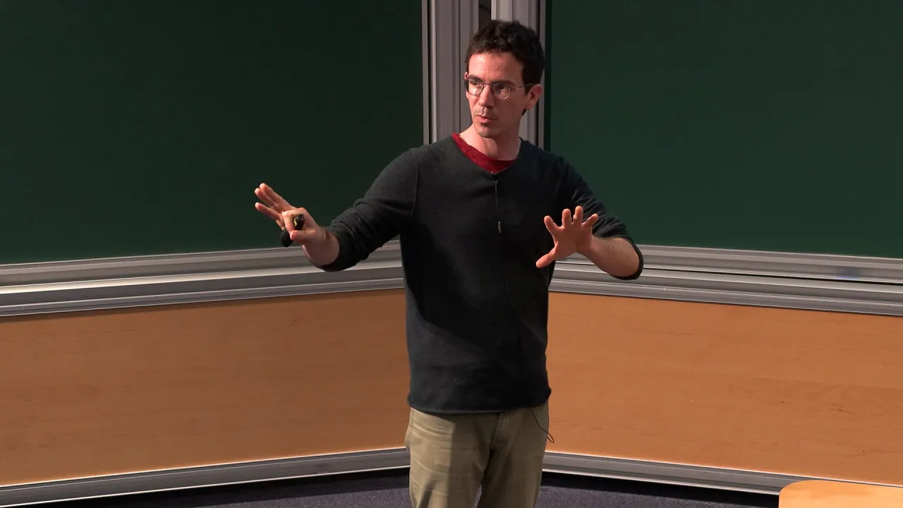


Rough paths theory, developed by Terry Lyons, provides a mathematical framework for handling irregular paths (like Brownian motion) where standard calculus fails. The key insight is that when approximating irregular paths, certain quantities like quadratic variation do not vanish, requiring additional data (iterated integrals) to be preserved in the continuum limit. This theory enables solving differential equations driven by rough paths by defining appropriate integration conventions (like Ito or Stratonovich), which is essential for applications in stochastic processes and physics.
Rough Paths for Physicists: Motivations and Young Integrals
Added:Basic Real Analysis: Familiarity with Riemann-Stieltjes integration, metric spaces, and the concept of Hölder continuity of functions.
Classical Stochastic Calculus: A solid grasp of Brownian motion, Itô's lemma, and standard Stochastic Differential Equations (SDEs).
Concept of p-Variation: Understanding how the variation of a path is measured, particularly the transition from bounded variation to p-variation.
Physical Motivation (Langevin Dynamics): Basic knowledge of statistical mechanics, specifically the Langevin equation and how noise affects physical systems.
Lyons' Rough Path Theory: Extending integration to paths with higher p-variation (p >= 2) using iterated integrals and the Chen relation.
Rough Differential Equations (RDEs): Studying the existence, uniqueness, and flow properties of differential equations driven by rough paths.
The Path Signature: Exploring the signature of a path as a fundamental algebraic object and its applications in machine learning and data science.
Regularity Structures: Advancing to Hairer's framework for solving singular Stochastic Partial Differential Equations (SPDEs) like the KPZ equation.
175 views0likes2:16:30Original Release: 2024-10-07
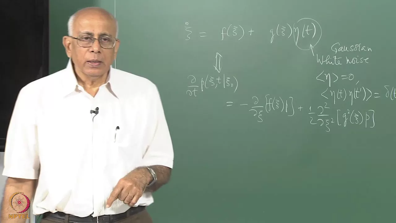
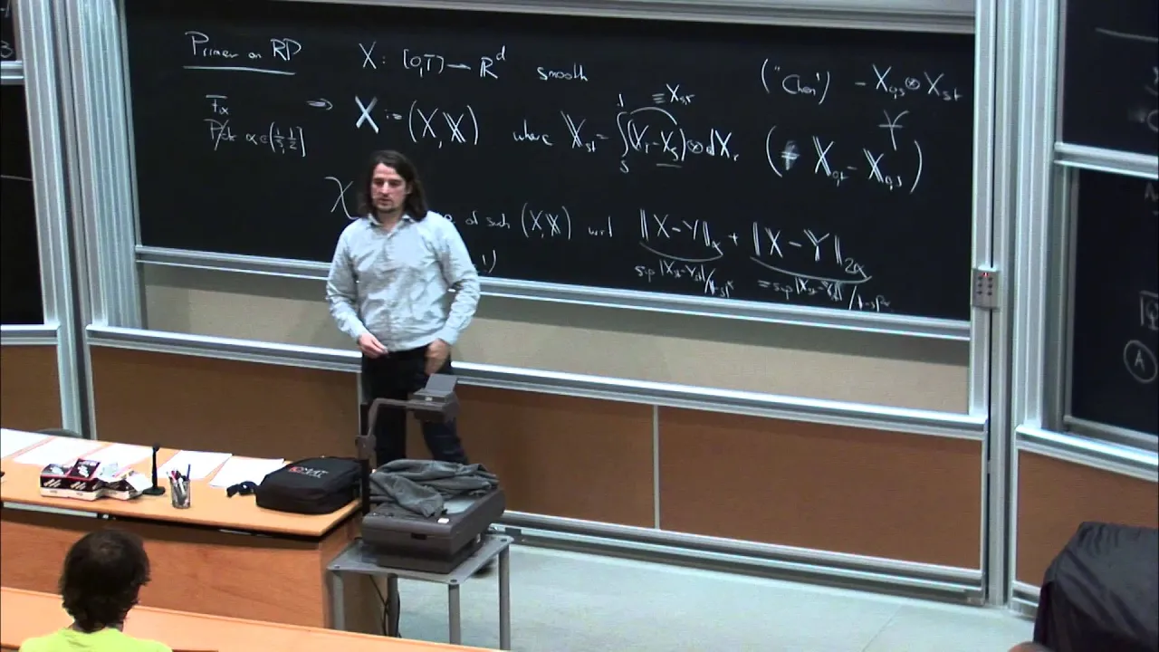
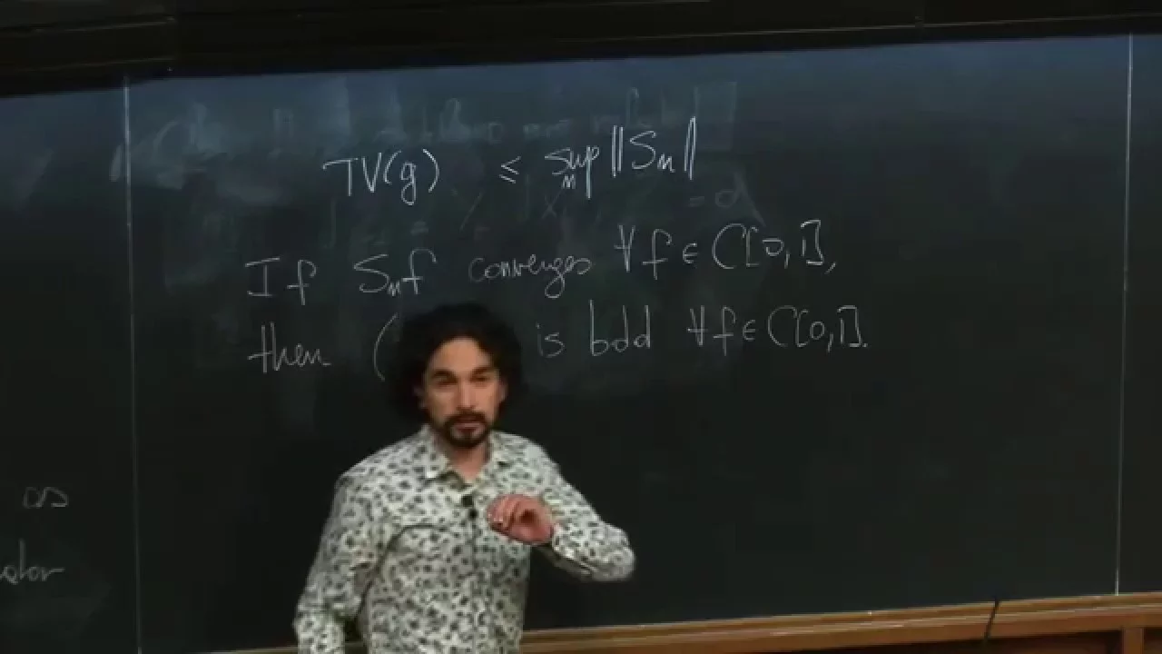
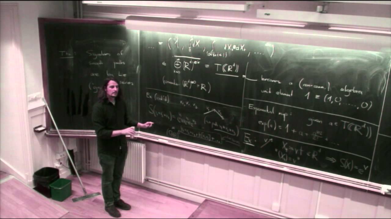
[Music] thank you good morning so um I will try to introduce you to some uh recent subject in mathematics which was born basically at the end of the second Millennium and the the main uh provider for the theory at that time was someone whose name is not very well known to physicist his name is Terry Leons he's not related to the French Leon's [Music] family okay so um why do I give these lectures first of all because um it's well it's something I think is rather new as I said and interesting and also because somehow where even if it's a mathematical Theory it it has some flavor of physics and I will try to insist on that and uh mainly I I what I will try to uh explain is that the intuition as that we have of the renormalization group uh is somehow find find what of one of its simplest uh Avatar let's say in raas theory so that's uh that's the uh first motivation for me to give the lectures um the another motivation is that when I when I first heard about a rough path it was maybe 10 or 15 years ago I really couldn't understand at all what mathematicians were saying and uh it was really hard I mean trying to read or listen to seminars and um of course after a while I started to think myself with the help of notes and it took me hours to understand what was going on even if in the end this is basically simple uh and once you've understood me as often often happens in physics or mathematics once you understand you realize that in fact what you did not well you don't understand why do why you didn't understand before uh so uh I decided to give a presentation which is rather different from the presentation that mathematicians usually give and I hope this will be helpful for some people so that they will waste less time than I did but I realize now that in fact the textbooks are excellent once you understand so either to start if you don't like my way of presenting or to get deeper I can refer you to two books which are essentially as far as I understand the the only text books so um let me give you the um I don't have uh so um there is one written by [Music] um hello and the name is the course on ref PA see it's Springer and the second one is uh the same first order and it's I think it's it's called multi-dimensional stochastic processes as ref size uh and this one is slightly more advanced and if you're interested in the subject you should have first a look at this one but this one is they both are very good and uh okay so what I'm doing will I will cover really a very small part of what these guys cover and I will try to be a little to have some originality which is I don't think it would be good or bad but it's it's supposed to be a bit of um as the subject is not very familiar I hope that will interrupt me as soon as I say something which is for you mysterious uh because uh that's the only way we I can keep you with me so don't hesitate to interrupt me and ask questions um so just to say how the lectures will okay so um to be concrete um I will try to put uh notes I don't know if there is an official way to do it but I have a web page a piece on the website of the lab which is When anybody can have a look at it and I will put uh we will relink it from the your course page and you have a course page will link to your okay perfect okay okay I can the dire okay so I will there will be a lecture notes uh at least for the first lectures I mean I realize that it's a big work so I I hope I will be able to keep the pace but okay not totally sure what I hope to do so um so what I will do today to start with so there will be uh a long in fact uh discussion of motivations and then I hope to be able to do it uh uh today Define formally ra but in fact once once we've gone through the motivations you will have a precise idea of what a rough pass is so should be okay and and then if really I'm very fast which I I'm pretty sure I will not be when then we will give the simplest examples if not today then next time and then we will spend I will not give a precise but then we will give an integration theory for after essentially and uh there will be a few uh well quote unquote physical applications and this will I will try to uh make things in such a way that the first hour will be the most demanding there will be concept and it will well it will it may be hard at some points even if it's not so hard and then the second part will try to give illustrations that's why I would be able to deal with the simplest example today but I'm not sure I will be but there will be essentially two main examples that I will try which are related to physics one that I call uh motion so you I will I will explain what this means but uh well it's it's about densing the vales as a bronan walker and the second one is uh bronan Motion in a magnetic field okay so this is this so this is for today and this will uh keep us busy for the next uh uh sessions uh this this is made of several parts and um I will get more details but today we shall focus on essentially on motivations so is there already a question I've said nothing but why not start with the motivation so uh this is I in fact I don't know if I'm right or not to do that way because this motivation section is going to be uh a bit well technical but it's basically simple so uh well why why not why not do it because it really leads to something important in the end okay so uh what what is the basic idea is essentially is that um in in mathematics and physics many things are defined via a limiting procedure if you start for instance thinking about even simplest simple things as R and integrals what you do is you do certain sums you take a limit and you get the integral and of course the sums you could explain basically to well any anyone 10 10 year old kid and then the notion of limit is a bit more demanding and there is some price to pay to get the integral but once you have the integral you can do many interesting things and in particular you can use integral to approximate sums and think of the ear M formula for instance or even even really really finite integrals and finite sums um and uh so there is an interplay between discrete objects rean sums and the continuous object which is the rean integral and if you think about it historically in fact before the integral existed but mostly it was seen just like as the anti derivative so you could Define the integral as the anti-derivative so the integral of blah blah blah is the thing that when you take it derivative gives the function and this was the view of mostly Oiler and and many well up up to Oiler and even afterwards but this has to be well this is not totally correct because Archimedes for instance computed volumes and surfaces and all that by by by splitting things and and essentially doing what we would call him sums but nevertheless for a long time you know when people were solving differential equations or whatever they had this view uh that uh this was uh really this was finding an anti-derivative even if oer used the oiler scheme that we shall come back to so so we could Define the integral the antiderivative but of course it would be a Pity not to know the relationship with sums and uh that that's that's another uh example that is probably familiar to you is the case of random works so you imagine you take the simple random work so probability one2 you go to the left probability 1/2 you go to the right and you study this this thing and again this is an extremely simple object to Define even if you can ask questions about it that are very hard to answer and it turns out that in fact if you look at this simple random walk or basically at any random walk with a second moment and you look it at it from far away well what you will see is an object in the Continuum which is bronan motion and again bronan motion is something which is more complicated to Define than uh the random work but at the same time it's much more flexible because it's in continuous time you can make changes of variables you you have itos formul just like that like you have had the change of variable formula for integrals which make them more manageable than sums exactly the same you have this object in the Continuum bronan motion which is much more flexible and you can use this object in the Continuum to prove things about random Mo which are totally non-trivial and to give just one example for instance the law of the iterated logarithm for random works is proven by first proving it for the B motion and then using some principles so there is some kind of interplay between random works and bronan motion it's totally possible to Define bronan motion as a limit of random Mo this as a definition of bronan motion but there is it's also possible to Define it well somehow more abstractly by giving saying that it has independent increments and that it's a gion process so the increments are motion and independent and if you see the definition this abstract definition that it's a Goan process with independent increments of course the relationship with random works is not totally visible to start with but it would be a Pity to think of Bron motion without knowing that it's related to random works okay so um now rafas Theory Falls really into this category that well let me say one more thing in fact basically as I said any random work with Vanishing mean and the second moment when you look at it in the large it's a bronan motion there is universality in this game and in fact somehow it's it's a remarkable fact that you can say something at many many objects by looking at only one and rafas theory is also something that is built basically to deal with such uh a situation and motivated in fact this is even simpler than random Works somehow it's just the following so you imagine that you have a certain uh object Q it's just a a function which goes from Ab let's say to R let r k so it's a function with K components so you have 21 2 K and then you can take um imagine that this one is but let's say it's continuous or whatever or integral let's say it's C1 so it's it has a derivative and then you can construct iterated integrals and those so how do I Define integrated integrals it's just so these are tensors and they are given by integrating or let's say let's do it on the full interval we could do it on a sub interval so we take K points I'm sorry S N Point points I'm not happy with that so let's call this one n and let's take K integral I prefer that and you DX i1 X1 DX I so if this is a if I'm sorry this is not an X this is Q this is this is what I call iterated integral okay and so this if Q is differentiable you define it just you take this as a definition somehow if you want it's just the integral d i1 over e s evaluated at S12 i k ds evaluated at SK D and you put the same bounds that's one this you take as a definition somehow okay so you have you have these objects at your disposal and now you can say okay now what happens in the following situation that you have you imagine you you are in a physical problem and there is some parameter you imagine that now that you have a family Q of Epsilon or positive Epsilon of smooth Maps I use the term smoooth for C1 for me if you do differential geometry usually what you call smooth is C infinite but what I call smooth is just C1 now smooth uh smooth maps and you ask what happens at small epyon and then it turns out that there is a whole zoo of things that may happen so the first thing is for first of all if sorry respect to EP or respect to S1 escape to S1 Escape they depend on Epson as [Music] smooth in s and so the first thing you would ask basically is the following that you would asset this which has defined as Q exists and of course as you know there for uh Maps or or path there are many many definitions of what a limit means but let let's take it very uh let's be very vague there is no need to be more precise at the moment and then well if it exists in a very strong sense of course things will go well but then but what about iterated integrals to assume so this is an assumption what about to do the and basically that's uh the uh the the the one of the sources of half Theory so before we tackle this let's look at something which is which is of the same kind but which is extremely familiar to all of us which is the following suppose you are in the plane as you will see I'm totally unable to draw a square but let's let's pretend I can I I draw the square and then I draw the diagonal okay and I would like now to approximate it using Y I'm sorry X Y well if you want X Y no I'm asking what is X what are the axes okay just anything okay yeah and I want to approximate the diagonal using a part on the lce so if the mesh of the lce is one the best I can do to approximate the diagonal is to do that so this is mesh one now if I use mesh one2 of course I can do slightly better and I can do this so if I have other colors excellent I could do I could also use the other side but okay so this is the one at MCH one half and then I can go on and of course if I do it uh let's let's do one more step you already see that I a bad drawer but anyway so let's do another step and you see that as mes as the mesh get small the path gets closer the diagonal that's and and in fact it even if you want to say things in in mathematical term it converges uniformly so really if if you look at the N generation you are never more than square root of 2 * 2 Theus n on the uh on the diagonal however and that's well I guess you all know what I'm wanting to say if you compute the length however the length the length of the L pass Remains Two instead going the length okay whatever you do you have to Leng to instead of square root of and of course you can imagine that imagine that there is any relevance to this situation that you have let's say well of course if you just look at the limiting uh approximation you would just get this straight segment and and if you would forget about this problem with the length you would lose some and essentially uh the analogy with rast theory in the limit keep track not only F the diagonal but also of the anomalous length scale so the limiting object would not be just the path but something telling you well beware when you measure length along this path this is not the canonical length in the ukan plane it's it * sare root of two okay so you keep both and then also make and then you make good use of it in applications so this is the idea of R but in many interesting situations you need to keep additional data in the Continuum to really keep what is essential in the discreet you cannot just get away and forget about all the uh details there are some details that you have to keep and this is this is really the the the simplest example that you can think of so let's return now one second data about two and in the diagonal or in the in the which one are you going to to mully the limiting object is going to be made of two things the diagonal and the square root of two in that simple case and square root of two being understood to be this the the anomalous scale okay ofan length is not continuous with respect to the convergence yes exactly so isn't there another notion of distance in the plane which not be variance in which length of the dional would be well you if if you you can choose whatever whatever1 well yes I I agree with you in the if you if you use the the norm which is the sum of the the sum not the square root of the sum of squares but just the sum of the absolute values so it would be the well what is it it's the L1 L Infinity in that case it's one of the two anyway yes it would give exactly that this one would be continuous we respect yes well but for for this simple example that I show but I'm pretty sure I could get it to be discontinuous for for other things yeah I I have okay but I agree I had in mind that I was I wanted to see this as a ukan plane with the usual distance and I'm just observing that sometimes going to the Limit doesn't behave way well with respect to integrals the distance is is obtained by Computing an integral and if I well and well I I've not thought about it but I'm pretty sure that with any notion of distance I could cook up examples in which convergence doesn't lead to to okay so what about itated integrals and then so you imagine that this exists and what can happen to integrals but then well this is as you may imagine it may you you have at least two things and they are somehow related that may happen the the first one is the following um so uh situation one um andum I'm sorry I will assume as well and assume assume that they converge as well so you have your Q you have this collection of objects and you assume that when you take the limit there all these things do have a limit and the situation one is the following you can have that the limit is smooth but the limits of itated integrals are not the limits the the iterated integrals integrals of the limit in situation two Q is wi enough the limit is wi enough but it's inter it's [Music] integrals do not make sense you see to make to to make sense naively of this object I had to say okay let's so I imagine this is smooth I can take the derivative and then I view this simply as as R and integrals but now you can very well imagine uh that um that the the even even if this limit here is taken in a rather strong sense not too strong but rather strong sense it may be that the limit is wild and and one one simple example is that for instance you can approximate on motion by by by part which are differentiable or at least P way is differentiable or by a by a random work whatever which is which you can view you can if you have a random work you can just view it as a differentiable except at the at the corners so so this would make sense for if Q was given by a random work and you would just connect the different steps by straight lines this would make perfect sense as well by you integral so you say Okay Q is the are smooth but then you use DQ so you integrated you are you are doing a derivative and then an non-derivative so to me it looks looks that you don't have an issue is because you multiply you have a multiplying derivatives well yes well we we'll see examples yes in fact the the the first the first r that I will show you will be one of these situations where Q is Q Epsilon is it's extremely simple so QEP it's something that is hard to imagine in one Dimensions you have to be it takes it first of all I have no issue when I take k equal Z in you CU I I would I would do integral of DQ from A to B and so that that would just be for me the difference of yes that's fine that's fine if you think about the next one it's already you're already in trouble that you have a multidimensional object or it's already if you don't have a multi-dimensional object you can always so you see you can always decrete for one dimensional object you can always decrete that this is qbus QA to the K divided by factorial of okay but but even in that case you could imagine you see this is this is fine but if the limit Q Epsilon of Q Epsilon is irregular it wouldn't these integrals wouldn't make sense at all I mean you wouldn't think think of it okay so let's answer this question how do you make sense so as as you mentioned the the first integral it's it's easy to take so imagine you want just to take the integral from A to B integral from a u DX V QV U this is the second integrated integral written slightly differently and I AG with you that it's hard to imagine that this should be something different from QA q u minus QA so this is integral from A to B 2 uus QA U and then well in that case I already at least if I well of of course I could decide that I take this as a as a value but if if I really want to compute it on honly if I don't have any regularity in Q I don't know how to do it you will see examples many examples but this is where yeah your Q DQ you cannot say that it's DQ Q Square well okay but then you okay I agree with you in one dimension you can as soon as you have two indices your loss okay but in one dimension you could but doing so is just like you're just in putting yourself in the position of Oiler which is not too bad which is that integration is antideriv derivation forgetting that what we would like to have is an independent definition of this object not something that it's the anti-derivative of something you see for oer the fact that the integral is the anti-derivative is a definition but after reman it's a theorem it's a theorem about what's it's a fundamental theorem of calculus yes okay so if you doing so you would put yourself in the situation of Oiler again I I would I would buy it immediately if you ask me but yes just a good question for the two situation we in both case we assume that I mean that for all K all order in the dimension they all have well well you you can you can imagine that you cut at some you could imagine looking just at at the at k equals 2 you you you just look at part of that and in fact that's okay so let's let's make already in fact it turns out that in many interesting situations what is interest what is important is just the first few of these guys and it's it's a situation which is very reminiscent in a somehow trivial case of what happens in Quantum field Theory when you have a renormalizable theory which means you have only a finite number of objects that you need to deal with and once you've understood them all well some finite number of correlation functions that cause problems and once you've cured them all the other ones you get for free of course Computing them is just another story but from the principles you okay you're only interest some simple integrals for example example you gave is the the length QE Square yes in that case we we we just look at these simple things but you can do many things by solving well by by integ you can already do many things okay and so somehow half the so you see that and and in this situation too it's also the case that you can imagine two different families qon they converge to the same q but iterated integrals they convert but they convert to different things so there is even well the point is that the relation between q and its iterated integrals it's somehow clear if Q is smooth if Q is not smooth you cannot just you if you just say okay Q is not smooth I just approximate it by smooth objects I I manage that the iterated integrals are defined have a limit and I take this as a definition in fact it's not perfect because if you do so you will see that this depends on the approximation scheme you've chosen for there is no Universal solution to that okay um before yes Z everything is fine is move there could be a situ zero where Q is Mo the limits of inter integral are the limits of yes sure oh yes sure but okay but then interesting I agree with you there is situation zero you are perfectly right I'm sorry you will give a some what you're going to say is a way to address situation one yes exactly yes and in fact I I address situation one and two in a way that in situation zero I do not do anything crazy so I I will give I will give a way to well I well half the gives a way to address these situations and and in fact if you apply it to situation zero it doesn't do any AR harmful thing [Music] um okay [Music] um so so what so the the main character in many things we are going to say are a few of these iterated integrals but we'll go to something which looks different which is called controlled differential equations and you will soon see that in fact these iterated integrals play an important role in that subject too okay so it's neveress if you have questions it's well maybe it's a nice point to to stop well you I can proceed okay so what is a control differential equation of course this is a complicated way to say something simple it's just you imagine that you are trying to solve something which is something like dyt is if I take my notation V of XT dxt and so I imagine that for instance X goes from a to a certain Vector space e and Y goes from uh AB so is known why to a certain Vector space f is the unknown and to make sense we view this V YT is a linear map for fixed for let's say V of XY is a linear is f x y linear map e f so I could put in this this and if I put indices so how how I named the indices in this uh so with indices this would be equivalent you will see so the if you think this is a little bit fancy so this would just be you would have Dy mu is equal to V mu I x d x y and if I I I will mostly use the Einstein summation convention that when I have indices down and up I sum of them let's put the summation so this is and this will be for me one D isal to the dimension of F and N is the dim menion okay so we it's is essentially equivalent for us okay so um so if if you think about it a priori uh this is well this is a Formula somehow but we have not made sense of it and one way to make sense of it when X is two again is that you define v SOA of YT and T we Define it just to be B of uh let's let's say T DT and then this equation will become equivalent to dyt DT is equal to B which is an ordinary differential equation we applying the same kind of trick as the one we applied here to Define these integrated integrals by saying that this is going to I'm just doing something stupid stupid this is the way to make sense of it but I would like to say that when I say that these two things are equivalent somehow I I do not really say something like that what I'm saying is that I interpret this equation as being that this is an interpretation I'm related something that is not defined a prior I don't know what this means and I relate it to something which is defined as soon as we've defined ordinary differential equations and just to give one example of you have a question yes I guess that you there is a Mis mismatch between V of X and Y and V on YX perfectly right it's not me also in the second uh in The Matrix form yes and I and I don't know yes I decided to put the way to put the W and by the way on the V you are missing the second argument no no it's t no no it you see I replace okay okay okay okay okay sorry of te so this is just sorry sorry this is not sanj this is was me wrong State excellent no did you're right to ask I mean it's okay so um let's give one example that we are all familiar with of this situation or all when I say all familiar many of us are familiar with it as an example stochastic differential equation equs so we would take XT to be the two dimensional which is BT and T B is a b in motion and then we would take we would get something like dyt is Little V of YT I think it's just I'm just giving an example and the second is Sig YT DBT which is this is called the diffusion okay so this is an example one of the one of the functions X is bronan the second one is time itself and I'm looking at this equation and this leads to okay so and then the way this is you dealt with is the following you say okay I'm going to to say that this is let's say little Y at time let's say let's imagine that I take t i just simple and then I would transform this equation into this which is integral from 0 to T V of y s d s 0 to t s but okay so just just to make contact so this is mathematicians and if you look at it from the point of view of physics you would say okay why B let's write it AST dot is B of YT plus Sigma of YT T and this is going to be a weight not and then the question is how do we decide whether this has a solution or not and mathematicians would say that this has a solution if there is some kind of solution to this integral equation so for that to be true those two things have to be defined and then you have to check that the left hand side is equal to the right hand side but you have to Define it so need needs to make sense and this is usually done by stochastic integration and I will make a remark let's say for the expert somehow which is that this defines this is not what we call a p passway definition so stochastic integration is going to approximate such objects by discrete ones just like the rim and integral but what we ask for the discretization is to converge not in the passway sense for every realization of R motion but in mean Square okay I do not claim that if you give me one bronan sample I'm able to exhibit you a solution what I'm saying is that I have the collection of all bronan samples I use it and I sure convergence in in mean I need disorder depends on time here so a discrete time formalism and you replace the brownan uh motion by random work That Is Random work yes then it would make sense uh yes that's correct yes that's correct um you're right but first of all it you will have to tell what you call Sigma and DV yes but but but but once you once you've told it it will be it will be yes you you you yeah um the point is that doing so is uh well again this would be going back to random Works whereas we we we agree that somehow Bon motion is is easier to manipulate you can make changes of variables and all that so for instance proving using discretizations that well you many many formula would beut but uh I agree with and in fact in fact it's it's even true that pawise that's that's correct I mean we in fact wait for wait for an example we we'll see what happens if you try to discretize these things yes question but if you do pathwise don't you get into these problems well I I will show you you have to give yes and I will show you how it works and and and and how it inspires what still that's that's one of the goals English thank you okay uh okay so to to say okay maybe it's wor saying it a little bit uh differently if you if you do stochastic integration you do discretization and what you say is that when you when the mesh is small you have a high probability that this is close to something which is not to say the same as saying that for any sample you go close to something it says that with yeah it's when the you discretize and you say okay when the mes is small there is a high probability that this object will be close to a limit and which is not the same as doing pass integation okay and in fact half pass Theory insists on Pathways constructions okay so the solution given which is very useful given by the stochastic integration is not the one raas theories after and it turns out that of there is there is a certain intersection on which the two approaches agree but there are things raas Theory can do that stasic integration cannot and conversely there are things stochastic integration can do that can do and it's 11 so I can sub here for the first it's we can stop 10 minutes yes starting from now so we will come back at uh 1110 yeah thank you and this uh motivates me to say be just slightly more precise here about what I told about stochastic integration so this is the following imagine so this is just a side remark in fact before I say that just from the what I will do here for Rath Theory and Rath integration and all that this is much less demanding than stochastic integration al2 this this is really an elementary Theory after that mathematicians have done deep things with rough PA but the the integration Theory and what I will tell you about is really Elementary and it's not comparable in complexity with it integration Theory from the point of view of the depth of mathematics so but nevertheless imagine that you want to compute something which is as simple as the integral from 0 to one of BS D DBS and you imagine that b is a b motion okay so if I want to be fair I would imagine that I have a probability space Omega and I have samples and I'm trying to compute this DBS of Omega so what am I going to do one of the possibilities for instance is to take the simplest discretization which is the following I imagine that I say that this is approximately sum from m equal 0 to nus1 of B taken at time m/ n Omega and making a convention I'm I'm used to Ito but making a convention in fact the point that a convention is needed is not so obvious but I I do it that way minus B m n I said that this is an approximation and of course these guys depend on Omega and now I can ask many questions for instance does this converge for a given Omega when n goes to Infinity so this is Pathways convergence so imagine that I call this I and I call this i n is i n of Omega going to limit for every Omega or almost every Omega so this is what I call pass ways and then mean Square is i n of Omega minus something Square okay so so I would like to take I'm sorry so I have this this probability space here and there is a probability measure here and this integral DP of Omega i n of Omega minus something of Omega s going to zero okay so this is what I call mean Square this quantity here could go to a limit when I fix Omega and I let go to infinity or maybe it fails to do so but nevertheless if if I look with so you see this comes gets small which means that with a high high probability i n of Omega is close to this object that I I just not really given a name to okay and so really uh what what rafas theory is about is trying to make sense of things in this for this situation okay sorry the second integral is a path integral now DP of Omega you can call it a path integral but this is a probability space and you have a probability measure so you integrate yes you could you could evate yes but so you you as a physicist you could see it as a br as a path integral but it's just you take the you take the expectation with respect to a measure and you have probability measure it's just like a just an ordinary probability space but in indeed as a physicist you might find a representation for this as a as a PA integral but here I just want to see I have a pro space I when I have a prity space it means that I have a way to measure things sets and we have a way to measure sets I can also integrate functions and that so that's this okay I hope this clarifies a little bit and if it doesn't again ask questions I mean that's I see that I'm already extremely late with respect to what I wanted to do but that's that's not an issue I don't care the the less I'm able to say the less I have to prepare for the next time for 100% benefits benefits um but I well I would nevertheless like to so um so I will uh look at one the one dimension the the 1D case 1D is very convenient because it avoids using indices and all that or using complicated notations it's a bit misleading at some points but nevertheless Let's uh forget about it so what we're trying to do is we are going we are trying to make sense of this simple thing the of course if you look at it this is just the same but this time x is just from a to R and Y as well and V is just a function from R to R this is very easy droing the yes just for Simplicity going to put it just for Simplicity because it again it simplifies things and it's it's quite natural in fact you will see this plays the fact that we do not include x there is plays a role in the discussions okay so now we want to try try to solve it via an iteration an iterative scheme and we are going to use ear so to use oer efficiently there is one very simple uh thing which is the following so imagine now that you have this object here and be extremely naive if f is a function apply the the stupid rules of differential calculus to get that d f of YT is going to be equal to uh I I hope I will do it right so this is going to be y so this is and go to an integral so this would tell us that F of YT going to be F of Y A if I start at a well okay let's start at S Plus integral from s to T F Prim of y u b of y u XU okay so of course as I've said nothing about the regularity of X this is problematic because I I have no idea of what this means at the moment okay but now I can say okay this is just mathematics this is defined who cares let's just say okay now I expect that if things are nice I can just if if s if s is close enough to T just approximate u v of U say that this is just just going to be equal to uh approximated by let's say F of f Prime of y s d of y s okay so get an approximation to get an approximation which is going to be that F of YT is approximately equal to F of YF plus integral from I'm sorry so now we're going to apply the Jer jerem rule that if this is a constant we take it out of the integral if we if we replace this by the value at s we take out it out of the integral and then we say that integral from s to T of DX dxu isal to XT minus X and we are led to an approximation so this is going to be frime of y s v of Ys um XT minus Xs and then if you imagine that a equals t0 let's say less than T1 less than TN less than b where going to apply this solve numerically to get F of M +1 is going to be equal I'm sorry F of Y at t m + 1 is going to be equal f y m plus F of y m v of Y TM xtm + 1us xtm okay so this is called the scheme and the question now is if I do that but then I refine this subdivision enough does this lead to a convergent uh so this is this I call this I call a subdivision Delta the mesh Dela I Define it formally but you say this is just the sub sub of M +1 minus tmals 0 nus one so this is just the subdivision and question is this convergent a convergent procedure when mesh data goes down to zero and if it works then we have a good substitute why bothering doing some complicated integration Theory I solve numerically and who cares and yes well I'm sorry I can no it's just it's just a way to um well I'm sorry you're right you you got a point what I'm really interested in okay so I i' I've mixed a little bit two things so what I really interested in is just do it for y so YTM + 1 is YTM uh then this this would be one so this is Y ym X + I do it for I I do it for this I'm sorry and the question is I'm your per that's a perfectly legitimate question and then this is this this this makes this makes sense but uh I don't know how to iterate it okay this one you agree I iterate thank you and again we've already come down to the one dimensional case but we will go to an even simpler thing which is the following just take example V of Y is equal to Y so it's the identity function okay so this is the scheme so we are saying that y t m + 1 is equal to YTM times one so this is the thing we are going to uh look at and the point is the following so so we shall make some an assumption it's that X is continuous XT is continuous in t Okay and then you can imagine that when the mesh is small enough we can estimate that XT m + 1us xtm is going to be an absolute value less than one so that this is always going to be a positive number and we can exponential it and so what we would so what we would get is that log y + 1id by y a is going to be just e the sum log I'm sorry m l I'm solving this equation Lal 0 2 - y 1 1 X um okay and then so it's a little little exercise with inequalities for instance so let's take it as the simplest one so okay so let's just let's just be rude that L one proex it's going to be uh if I say something if I'm not to and I subtract X and this is going to be larger than minus X2 and this is to be smaller going to be smaller than minus X2 over 3 this is crude and this is valid let's say how do I say so imagine that this is you take X in absolute value less than 12 so this is a little inequality and then you see that this sum here so what do I get I get that YTM divided by y a is going to be e to the x t m minus XA plus something and something is [Music] between z uh to- x l + [Music] 1 x l - 13us x so this is power two this is this okay this is it okay so now you see we are facing a a little problem which is what happens to this guy and now we are going to use a little theorem that is maybe not so well known is that if x is a continuous function there are subdivisions Del is small mesh which that Delta is as small as we please and Q Delta I'm sorry Q Delta is Define it to be this I put a little index M sorry will Q Delta this leads me to Define q Delta is just equal to sum from 0 to n minus one you see this the more the more points I if I add if I increase M up to n this is going to be increased so let's look at this one just the last one so you see if I'm in this situation it's the sum from M = 0 to nus oneus t m okay so now I use this little theorem I can give you a reference for it so this can be arbitrarily small so you see I can find subdivisions for which this is very small for which this is very small so this is well approximated just by xtm minus XA and then either this holds for any subdivision which with small enough uh mesh and then I'm happy or it doesn't hold and then I'm lost so there is a dichotomy deine good well so if this is called the quadratic variation so if the quadratic variation goes to zero when mesh goes to zero then uh what we get is that YT is going to be y y a e to the X cus x a is a limit on the other hand if this guy if not then you see because of this uh this let me uh because of this bounds um you see that there is no way you will be convergent because for imagine that there are subdivisions for which this remains larger than some some Epsilon even if the mees of the subdivision is very small then this is going this this here is going is going to prevent convergence I know that for certain subdivisions I can make this extremely small and then this is the only POS this will remain but if there are some for which this doesn't get arbitrarily small then I will not know where I will is itate between one what should I take here okay so if not then there there may be no limit there may be no limits CH choosing different sequencies of subdivisions may lead to different results of not result at all okay so uh you see the question now is so what what can we do X does not have quatic variation and the answer is well let's try to go one step further let's try to do an improved approximation qu variation does not go to zero smallish I should call it the two variation in fact if I would be um yes because if you have a subdivision you can apply it to each part of the subdivision so you see yes I assume that it was continu I said it somewhere assumption XT is continuous in t well the problem is that if if it's not true that Q Delta is small for every subdivision when the mesh is small then you do not know which subdivision to choose to make your computation does that answer your question what what I'm saying is that it's only the only possible the only possible limit for this equation if there is one is that this is the solution and this can occure only if uh X is Vanishing if not I will be able uh to equal if not I will fail and it would of course you could say Okay I I take my X and I take only subdivisions for which it works but this would be extremely inconvenient I mean if I change x a little bit you will you are lost and you have to start again your computation from not no exactly there are subdivisions for which is very small which means that the only possible limit is zero it's not possible there is no function for which this has a limit which is non zero if there is a limit it's zero and I I I will in the note you will find some observation you might think that bronan motion is a counter example but is not motion has Vanishing B motion doesn't Okay so maybe I shouldn't have said it at all where is my so let's do let's do it so let's let's go let's continue this example and imagine now X is a bon motion then it's an easy computation that if you compute so let let me just take a notation so what I so let's do this computation quickly so imagine that that this means that XT minus XS is an N minus s0 go R variable an independent of non overlapping other increments okay so this so the only thing we have to know about it so we have that the expectation of XT - XS is equal to zero and the expectation of XT minus X s² is equal to tus s okay and I use this notation expectation the physicist would write it as average XP minus Xs is equal to Z blah blah blah I use the the mathematicians notation expectation and another way to write it this would this would can also be written integral DP of Omega X of omegaus x s of Omega Zero have a probability measure I can integrate with respect to this measure this is integrate the temp Omega okay so then it's easy to see that for Bon motion Q Delta of uh X this is equal to B minus a because you see for each for each little so this is sum from M 0 nus1 n + 1us TN this isal to B A and if you work a little bit using the properties of uh gos it's easy to see that the odd moments vanish and you the only thing you need to know for the rest is that of this computation is that if I take the power four this is equal to 3 tus s squ and then you will easily see that e of U Delta of x minus b - A squ I guess it's just if I'm not mistaken two some from n = 0 nus one uh m + 1us m s with a little compensation if you don't see okay and so in particular this is less than twice B minus a mes of Delta so this is this is really if you've never done this computation do it for yourself it's easy you use the fact that the indep the increments are independent over nonoverlapping intervals so typically yeah this is easy okay and so which means that so this is an example of uh convergence mean Square Delta converges to B minus square and okay but do conver to zero no converges to B minus a no so it's we'll see wait a see okay so this is it and in fact from this this is a standard okay so so this is an easy computation and then there is a theorem it's a general theorem of probability that in fact if Delta N is a sequence given in advance of subdivisions with mesh Delta n going down to zero then uh Delta of X converges B minus awise okay almost short if you want okay so imagine so what you could say is that at least when X is Bon moot when X is Bron motion it would be tempting to say okay in fact I can use this theorem whatever if whatever uh subdivision I use so then in fact if you ref if you refine if you if you look at it um when X is small so let's me just f EP than zero when X is smaller than some Delta of Epsilon then in fact the log of 1 + x - x is less than minus 12 1us x² is larger than 12 1 + x² okay so this is just a refinement of the uh little thing with said before and so if you apply this result you will see that it seems that in fact what you get here is 12 minus a when motion and in fact this is to be taken with a grain of salt and the point is the following the point is that if Delta n chosen arbitra is chosen in advance this is okay but one can given Omega cook up subdivisions such that Delta is arbitr [Music] small that was my previous statement that you can you can always cook up uh subdivisions with arbitrary small mesh such that this is arbitr small but also others such that Q Delta is arbitr large in fact so this is again the phenomenon we know very well in physics it's just in inversion of limits somehow if I take Delta in advance then I can choose essentially any bronan sample and it's going to give this result however if I'm given the bronan sample but I'm unlucky enough to take a sequence of subdivision which is bad this will just oscillate between zero and infinity okay so fix subdivisions take a br sample that's fine fix the bronan sample and be take a bad sequence of subdivisions this will explode this will not work okay so now the question is what can we do and there is something very suspicious about this result somehow if you think about it it's that this result here is typically what you would expect from applying uh eastic calculus somehow but you see we manipul ated everything as if we could use the standard rules of differentiation want the Quadra variation which is precisely yes that's correct however uh you should does not the point is that I you well maybe this will be clearer but not today because I don't have time oh yes I still have well okay we'll see um no the the miracle that leads to this solution is just that the older scheme goes forward in time we we really apply the the scheme implements the convention without saying it so but but this is nevertheless this is very suspicious so what can we do if x doesn't have aning variation and I have to go back to my previous formula and uh you see I had I had this formula telling me that F of Y is equal to F of y s plus um integral from uh s2t F Prime [Music] this was my formula but of course I can navely iterate it now you see this guy here is again of the same kind like I app appli the same formula to it and then what I get is that F of YT is equal to F of y s plus integral from s to T F of fime of y s v of y s [Music] uh okay I have to uh concentrate myself a little bit integral from s to u f Prime of y v so it's becoming becoming a little bit messy so let me take the formula just to be sure that I make new mistake I prefer to have a look it oh so know I I wasn't that I wasn't that bad F this is you see I'm applying the formula for f to this big guy here so I take this guy here and I take his prime just like I to the prime here and then we B of y u this is the guy x v and here I still have my dxu you see iate and then again I play I okay so this one I can take away and this is this is this is just giving me back my first approximation and here again I approximate here s what I get is then that I have y of YT is approximately equal to Y of y s plus fime of y s v of y s x XT minus XS this is my previous approximation I get a new a new order in my approximation which is this big thing here that gets out of the integral so um so let me just a bit short fime V Prime V evaluated s the integral from s less than V less than U Less Than t d x v dxu so this is one of our integrated integrals okay so now you see we are so first of all if x is smooth then the usual scheme is convergent as mes of Delta when mes of Delta goes to zero and the improved that the second order scheme so which is which would be this I call it the second order scheme this one would be better it would con is convergent mesh Delta Square when Dela goes to zero this integral makes sense and U and we are on the safe side and now comes the uh somehow good surprise what if if uh X is not Smo the first possibility in fact the naive or smooth uh X is integral dxq dxv dxq from uh s this v u e this is V this is 12 uh X - x s why not take the for why not take the same formula and then if you do so again so the approximation you see would be this and then you use inequalities bounds for log 1 + x + x² 2 - x so this is a big O of X cubed as you know but you can do bounds and then this shows that taking y t m + 1 equal Y TM * 1 + x t m + 1 - XM + 12 x t m + 1 - x m this is for the example Dy = to V DX leads [Music] to convergence proceed as soon as X has zero three variation what do I mean by three variation it's just sum of x t m + 1 - x t m cubed m = 0 to nus one goes to zero when Delta go down to zero where should have okay so this a converion procedure as long as this is and the result why isal to y a [Music] Theus and you see and I insist again we have used this time we really have used standard computation of derivative because even if we didn't really start with use uh well you see in this formula we really use several times na differentiation to establish this formula okay the in the but in the end uh we have the happy result that when this is uh small when this goes to zero and then it's a simple exercise to do the following you can go of course as further As You Wish is the following you you iterate the bone expansion use the formal rule that integral blah blah blah S1 SK uh b x S1 d x is equal to one factorial of k xbus x a to the K this is a formal rule because yes y y Aus a expression what do you do with quadratic term well you take the because when you take the log this is going to be eaten because this is the beginning of the exponential this you see this object here is is so you iterate the born expansion with the rule that this is true and then show that if x has Vanishing K variation I do not Define formally but it means to be the K variation here is the three variation the two variation was before I guess you can generalize 2K easily then the uh Okay order scheme is conver for Dy = y DX is convergent and YT is equal to y a e to the XT minus x a so this this is you see this is a good thing if you decide to okay so one point is that the higher this number is the easier it is to have zero variation with respect to this number so if you have Vanishing two variation you're sure that you have Vanishing three variation this is Trivial and then four variation and whatever so and this is reassuring because imagine that you you go too far in the born expansion and you make the computation you still get the same answer at the end there is a minim there is a minimal thing to do to get a conversion scheme which depends on the how wide X is but as soon as you've reached a level of approximation for which the K variation is zero then if you go one step further one step further one step further you can but you do not change the final result anyway you will find this that this is the solution so I it is natural that I take two more minutes Ricardo if you don't mind yeah I just wanted to ask you stupid question why do you call this BN expansion well this is exactly the born expansion if you if you imagine you have a potential in in the quantum mechanics and you iterate uh okay this well I call it the Bor expansion yeah okay this is a name I agree it's just because it looks familiar to me okay so I take two more minutes for the following remark you have up to five minutes okay fine it's it's more than enough X motion has Vanishing three variation but e tells me that integral uh v u B uh V DB U this is equal to- 12 BT - b s s minus 12 t - s so this is the stochastic integral what if I use this if we use this for the second order Oiler scheme so this integral is not defined Pathways you you do this this thing of what I exemplified on the uh other Blackboard of convergence in mean squ but in mean Square this is the correct answer so what if we use this for the erer scheme and the answer so so basically what you are going to use is now this y t m + 1al to YTM and this is going to be 1 + x d m + 1 is x t m + 12 x m + 1 - x I'm sorry xal to B it's x x and then- 12 t m + 1 minus TM well you see without surprise I'm adding this term but this is not going to this is going to count as little as it can and answer the sequence of approximation converges converges but this time for any sequence of subdivisions Pathways we don't YT isal to y a t the XT minus x a - 12us A so you see you can view this as of each integral I I've done the integration naively I've decided that this is this okay this is just naive integration and I do the iterations and I get the stratonovich solution I get a naive solution but if I say okay Ito tells me I should take this for the iterated integral what happens well fair enough what I get at the end is that the solution of my differential equation is again the EO solution so to summarize because my five minutes are over if you work with Bron and motion and you stop at the first oil scheme you find under some restrictions and by some miracle you find the EO solution even if you've made all the computations very naively so did not use stochastic calculus whatever however if you go to second order Oiler scheme if you use the stanovich convention to compute this guy you get the stratonovich solution and it works F wise and if you use the EO formula for this guy then you find the EO solution for this equation and that's what you wanted so the moral is that when X is irregular there is no a prior me that can be given to this conventions can be made and depending on the conventions you get different solutions for the equation I think I should uh questions in the room or in the virtual room the message is that at some place you have some arbitrary conventions to yes this you cannot avoid yes and it's a and from the naif point of view I want to have this is exactly as in Quantum field Theory you have your Quantum field Theory there is you have the Rel nothing is going to tell you what the mass is going to be in the end with respect to the bare parameters in your theory you have to fix it you have to fix the normalization of whatever wave function whatever and then you can have an answer but you need to fix things you need to F fix certain normalizations yes the number of things you need to fix is the order of the scheme yes yes yes for the second minus one for the first order there is the JY rule that we are not going to violate that the integral of DX is X this is this we not we do not you do not dispute yeah we knew that yes exactly I I don't exactly know how to say my question but it's more I'm surprised that for X where you you it's not smooth so you you have different ways of of picking how you should Define the integral yes and there we saw that for any order we get the same I mean if x is has the if you have to go to the case order to but you have to the it's the case order but if you get the same solution as soon as you decide that this is your definition then yeah what I mean is that you get the same solution for all this kind of I mean you don't you get the stratov one and not Theo yes so is this I mean so that means maybe there are some class of way to define your integral all similar to give you the same solution yes the point is that okay so we we shall come to that in the next lecture but in fact so another way to say things is you you see I I had this formula for the second order of course aray now but I had this formula for the second order I didn't know what I could make with the uh uh iterated integral so I could say okay let's let's approximate this path which is not smooth very smooth path and see what happens and then I could get essentially anything for this guy essentially say and then next time we shall uncover some important thing that this thing will satisfy whatever the definition if I take Ito tranovich or the limit of what what what take the limit of the sequence of smooth function whatever I do this here will have to satisfy a rule which is called the chain relation which is very important and which is well which is we shall start with it on the next so there is it's not arbitr there is arbitrariness but not complete arbitrariness just as in Quant field Theory where certain things are arbitrary but satisfy some consistency relations M you have written question written question where is it from the the okay uh well the point is that when you do the exercise of taking the exponential expanding and blah blah blah you will see that for the scheme to be convergent it is enough that uh typically X has Vanishing three variation which is true for B motion in fact but so the point is that you see usually if you take smooth functions and you take higher and higher order AER scheme you get something which is better which has better and better convergence properties because in N steps if you have an if you cut your interval in N steps typically if you take the first order convergence is 1/ n second order it's one/ n squ blah blah blah so you get better and better here ENT a similar thing happens things get better up to a point where well before a certain point things are not convergent and they become convergent after after you've chosen enough an high enough order of for approximation and then it stabilizes but uh we relax the smoothness condition just when we see that when we compute what happens this is convergent even if X is not very smooth but is only only has Vanishing three three variation or what this does this answer your question Domino you don't really need to have any probability this is just analysis this is just yes because yes no sure who cares it it turns out nevertheless that bran motion is typically uh well continuous object well it's it's typically one of these examples where raath Theory would apply and in fact one of the big successes of raas theory is of the descendant of raas theory which is called regularity structure and this is how mathematicians have are now able to tackle partial stochastic different nonlinear partial stochastic differential equations so for in the kpz K equation has been now the existence of solution and how they should behave and and the fact that they are indeed given by the naive uh L transformation what what's the name of this yes of course transformation is now a theor in mathematics and this is really one of the uses of so the point is that indeed there are other applications of rough pass than to stochastic processes but stochastic processes give just the the the nicest examples where you can apply it yes maybe it's naive I'm doing too much too many shortcuts but if I look at the formula of the log this you see that if you have the log of 1 + X+ X you keep all the terms you have log of exponential of x - x so you have zero so you have something I mean if you had X that has oral order in K so never vanish in K I feel like it would still give us a finite result it would still give us something so um well um okay so in that case that's fair because it's well I have chosen really a very very simple differential equation if if if you start trying to do the same thing for instance I'm asking that V has some reg the the one what I use this here when I write down DX Dy is equal to V DX B of Y DX when I when I go when when I do my approximations so if I look at the first order erer scheme I don't have to make much assumptions on V but as at some point I next time I have to take a derivative of v a second derivative and all that so in the end if I want to do what you want to do you have to assume an ticity in v and essentially you you would say that that V so you you would rewrite it dy over V so we could do that in one Dimensions as a d y DX integrate on both sides this is just V of Y you could decide that the solution so this is something you could do but in fact it's a it's a dead end if you go to higher Dimensions or for well for many reasons and and and again this would be like going being back there are many people who would like to be oer in this room but there is only one oer uh this is just saying that integration is anti- derivation which is not the procedure we want to have we want to have an iterative procedure with discretization to build integrals and then we have a fundamental theorem of calculus we don't want to throw away half of the theory Does this answer your question do you have theor to state that the Kate variation is uh more without Computing it to control the the Kate variation without Computing it well uh first of all if if your function is differentiable it has van ing two variation Vanishing whatever but apart from that it's just somehow your question is to me looks a little bit like is there a way to know that a function is differentiable without Computing well it's a bit of the same kind I mean no I I well older okay easier sufficient condition X is uh uh Alpha older with Alpha quickly larger than P that's easy X has Vanishing varation so this is a little bit easier to to check maybe then doing because this this you here you have to make a complicated sum here is this is something you can just verify locally it means that if you come close to the point so XT minus XS is bounded by some Kus s Al so this is something you can uh maybe check in an e easier way okay thank you today okay thank you
Up Next
52:32
Stochastic Calculus: Ito Integral Definition & Properties
@keesoosterlee4481
209 views•2021-05-14

4:43
Elliptic Curve Cryptography Explained: ECC, ECDSA, ECDH
@PracticalNetworking
28.5K views•2024-10-21

10:44
Fourier Series Introduction: The Big Idea Explained
@DrTrefor
387K views•2021-05-03

6:00
The Mathematical Impossibility of Accurate World Maps
@Vox
23.3M views•2016-12-02
Related Study Plans & Knowledge Roadmaps
Structured learning paths in Mathematics
mathematics
Tensor Calculus: Vectors to Riemann Curvature
01Mathematical Foundations: Linear Algebra & Calculus
02Covectors, Dual Spaces, and Tensor Basics
03The Metric Tensor and Index Gymnastics
+ 2 more learning modules
40h5 modules
Explore Roadmap
mathematics
Gödel's Incompleteness: Logic, Proofs & Limits
01Introduction to Formal Systems & Hilbert's Dream
02Set Theory, Cardinality, and Cantor's Diagonal Argument
03Arithmetization and Gödel Numbering
+ 2 more learning modules
14h5 modules
Explore Roadmap
mathematics
Galois Theory: Fields, Groups & Solvability
01Foundations of Abstract Algebra: Groups & Fields
02Polynomials & Field Extensions
03Splitting Fields & Symmetries
+ 2 more learning modules
24h5 modules
Explore Roadmap
mathematics
Non-Euclidean Geometry: Models & Geodesics
01Euclid's Fifth Postulate and the Birth of New Geometries
02Hyperbolic Space and the Poincaré Disk Model
03Geodesics: Defining Straight Lines in Curved Spaces
+ 2 more learning modules
15h5 modules
Explore Roadmap