















![Complex Analysis – II: [PART 4] Special Linear Fractional Transformations GGSIPU 2025](https://i.ytimg.com/vi/7d5RTcv6Xjo/hqdefault.jpg)



![대수학의 기본정리 증명 [2/4] 코시리만방정식~코시적분정리](https://i.ytimg.com/vi/86myNc_Ipqs/maxresdefault.jpg)
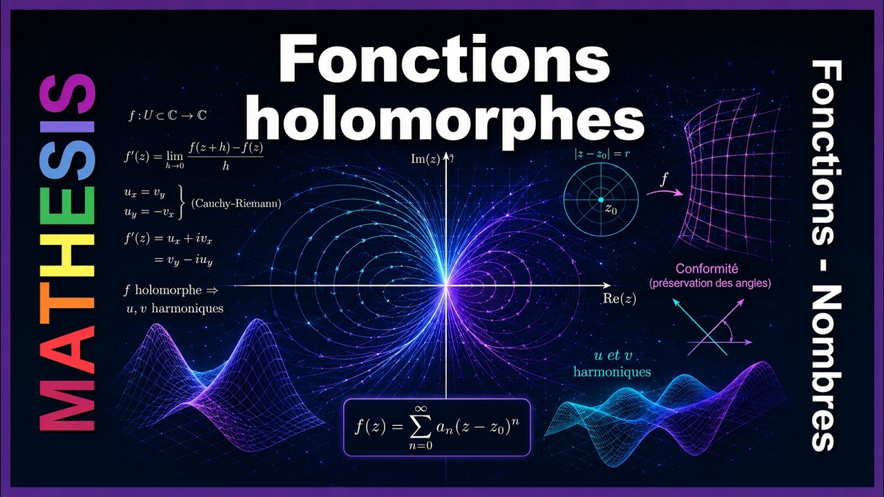
The Cauchy-Riemann equations are two partial differential equations (∂u/∂x = ∂v/∂y and ∂u/∂y = -∂v/∂x) that must be satisfied by the real and imaginary parts u(x,y) and v(x,y) of a complex function f(z) = u + iv for it to be complex differentiable (holomorphic) at a point. These equations arise from the requirement that the Jacobian matrix of the corresponding real function f: ℝ²→ℝ² must represent complex multiplication, which imposes the specific symmetric structure [[a, -b], [b, a]] on the matrix, thereby connecting the two notions of differentiability in complex and real analysis.
Complex Analysis 6: Cauchy-Riemann Equations Explained
Added:The representation of complex functions in terms of their real and imaginary parts, i.e., f(z) = u(x,y) + i*v(x,y).
Multivariable calculus concepts, particularly partial differentiation and the definition of differentiability for functions from R^2 to R^2.
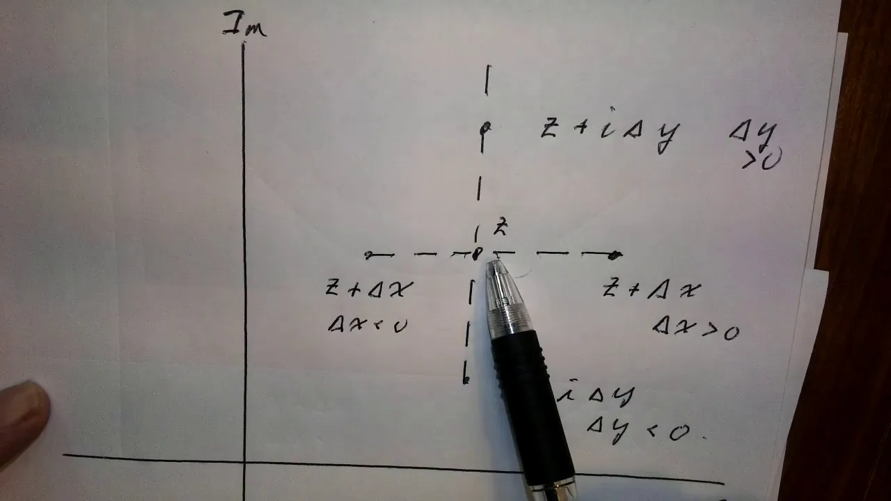
The definition of the complex derivative and the geometric understanding of limits in the complex plane, specifically approaching a point from infinite directions.
Holomorphic and analytic functions, including their unique properties and significance in complex analysis.
Harmonic functions, Laplace's Equation, and finding harmonic conjugates using the Cauchy-Riemann equations.
Conformal mappings and their applications in mapping complicated geometric domains to simpler ones in physics and engineering.
Cauchy's Integral Theorem and Formula, which build directly upon the differentiability conditions established by the Cauchy-Riemann equations.
48.5K views1Klikes12:39Original Release: 2022-01-18
hello and welcome back to complex analysis and you might already know first as always i want to thank all the nice people that support this channel on steady via paypal or by other means now finally in today's part 6 we will talk about the cochi riemann equations in order to understand them we first have to recall the two notions of differentiability we have for a complex function the first is the normal one the one we introduced at the start of this series this one we simply called complex differentiable at the given point z0 now as a reminder in other videos i already explained the domain here doesn't have to be the whole complex plane c it's sufficient to have an open subset however this might be distracting in this video here therefore i always write c for the domain so if needed you can just substitute this domain with any open subset u okay back to the differentiability here this one can be described as a linear approximation in c more precisely this means that we can find a complex number we can call f prime of set 0.
indeed this could be any complex number then with this it's possible for us to write f of set as a linear term plus an error term and you already know everything happens locally around zero therefore the constant term is f of zero then next comes the linear map which has a slope given by f prime of zero more precisely we have this number times z minus zero so you see again this is the linear approximation of the function f around the point zero and please recall in real analysis this represents the tangent therefore the only thing missing here is a corresponding error term we could call phi of course this phi is also a function from c to c now as an error function this map here should go to 0 when we send z to z0 and this convergence to 0 should go faster to 0 than the linear function would do or more concretely phi offset divided by z minus that 0 should still go to zero when we send z to zero now with this property we really get a linear approximation around the point zero indeed this is what we could read as the definition for complex differentiability at the point zero however to be honest it looks a little bit different than the definition we gave before yet i would say it's not hard at all to get this reformulation from our definition and i guess it's a good exercise for you to think about it after this you see we simply can take this for the definition of complex differentiability and that's a good thing because we can nicely compare this to the definition of total differentiability we explained in the last video as a reminder this definition we introduced for functions from r2 into r2 and there please recall we have a one-to-one correspondence between functions from c to c and functions from r2 into r2 therefore often both functions are just called by the same name f however to distinguish them i give the last one here in index r okay now we can recall the definition of total differentiability for such functions also there we have to fix a point in the plane so let's call it x0 y0 then we know the function is called totally differentiable at this point if there exists a matrix j and an error map phi please note i use another variant to denote the letter phi here then what we need is also a linear approximation now given by this matrix j and lastly of course this error term here should also go to zero in the same way as before which means if we divide it by the length of the difference vector we still get out zero in this limit here please note before this zero was the zero in the complex numbers and now this zero is the zero vector in r2 however using the identification c with r2 you could say they are exactly the same therefore a natural question here would be where exactly is the difference between both notions here so i would say let's try to spot all the differences first this might be obvious in the second case we see when we use the division here we need the length of the vector this is what you know we can't divide vectors however in the complex numbers we don't have this problem we simply can divide one complex number by another one now maybe this is not a crucial difference because both things just explain that the error term goes to zero and of course if we wanted we also could use the absolute value here indeed this wouldn't change anything for the linear approximation here therefore we have to look at the linear approximations to see the differences since we immediately see that the constant terms fit we look at the linear terms here and there you see this start here stands for the multiplication in the complex number c and that's the difference because this multiplication does not exist here indeed what we find here is a matrix vector multiplication now exactly this does not translate in general to the multiplication in c therefore the conclusion is immediately this definition here complex differentiability is much stricter than this definition there and now in order to get the translation from the complex definition to the one in r2 we have to answer one question namely in which cases does a matrix vector multiplication represent a multiplication in the complex numbers now because we know how to calculate with complex numbers we can answer this question without any problem just let's check how the multiplication in the complex numbers looks like so we take two complex numbers w and z and multiply them of course here w and set have a real part and an imaginary part respectively therefore we say w is equal to a plus ib and set is equal to x plus iy and now we just do the multiplication where we use that i squared is -1 then we get a times x minus b times y plus the imaginary part which is b times x plus a times y of course this was not hard at all because you know how to calculate with complex numbers however now we want to rewrite this as a matrix vector multiplication and the vector should represent the complex number z which means we have x and y as the coordinates and on the left of it we have a 2 times 2 matrix where the numbers a and b should occur and indeed how the entries exactly look like we have to figure out now and of course this is no problem for us because we already know the result the first component should just be the real part here and then the second component is just the imaginary part and now the question is which 2 times 2 matrix brings us to this result now the first row we see immediately because it should be a and minus b of course in the same way we also see the second row which should be b and a and indeed that's it this is the matrix that represents the multiplication of complex numbers therefore our conclusion here is if we want complex differentiability we need that the jacobian matrix here has this form so i would say let's fix this important result with a theorem in fact in this theorem we will now find the cauchy riemann equations okay in order to get everything together let's start with a complex function that should be complex differentiable at a given point zero and now we can just split this point into a real and an imaginary part and as before we call them x0 and y0 respectively so with the reasoning from above we know that this statement here is equivalent to the statement that the corresponding real function fr from r2 to r2 is totally differentiable at the point x 0 y 0 and that the jacobian matrix at the point x x0y0 has the symmetric form from above so there you see this is our final connection between both notions of differentiability and exactly this connection now leads us to the cochi riemann equations we simply get another equivalence when we use the fact that the jacobian matrix has partial derivatives as entries however in order to do this we have to introduce new names for the components of the function fr that's no problem at all because we know we just have two components the first one we simply call u and the second one v now both components depend on the two variables x and y therefore we simply write u of x and y and v of x and y in other words here we have two new maps that send r2 to so please don't forget here we just have real functions ok and now we know from the last video that in the top left corner for example we find the partial derivative of u with respect to x and now you see with the partial derivatives in the jacobian matrix we find a connection and exactly this connection is what we call the coshi riemann equations they are just two partial differential equations for u and v in particular the first one is simply that d u d x is equal to d v d y so here you see this equation just represents that we have the same number in the top left corner and in the bottom right corner okay and then you might already see it the number b here gives us the second equation which is d u d y is equal to minus dv dx and of course both equations have to be fulfilled at the given point x0 y0 okay now you know that we have these two equivalences to describe complex differentiability at a given point and of course then we can extend that to a whole open subset to talk about holomorphic functions in other words a holomorphic function has to fulfill the cauchy riemann equations at all the points okay then i think it's good enough for today let's talk about examples in the next video therefore i hope i see you there and have a nice day bye [Music] you
Up Next
9:53
Euler's Formula Explained: A Visual Intuitive Guide
@betterexplained
136.3K views•2010-07-18

4:43
Elliptic Curve Cryptography Explained: ECC, ECDSA, ECDH
@PracticalNetworking
28.5K views•2024-10-21
8:22
Laurent Series Explained | Complex Analysis
@brightsideofmaths
52.4K views•2022-04-06

6:00
The Mathematical Impossibility of Accurate World Maps
@Vox
23.3M views•2016-12-02
Related Study Plans & Knowledge Roadmaps
Structured learning paths in Mathematics
mathematics
Tensor Calculus: Vectors to Riemann Curvature
01Mathematical Foundations: Linear Algebra & Calculus
02Covectors, Dual Spaces, and Tensor Basics
03The Metric Tensor and Index Gymnastics
+ 2 more learning modules
40h5 modules
Explore Roadmap
mathematics
Gödel's Incompleteness: Logic, Proofs & Limits
01Introduction to Formal Systems & Hilbert's Dream
02Set Theory, Cardinality, and Cantor's Diagonal Argument
03Arithmetization and Gödel Numbering
+ 2 more learning modules
14h5 modules
Explore Roadmap
mathematics
Galois Theory: Fields, Groups & Solvability
01Foundations of Abstract Algebra: Groups & Fields
02Polynomials & Field Extensions
03Splitting Fields & Symmetries
+ 2 more learning modules
24h5 modules
Explore Roadmap
mathematics
Non-Euclidean Geometry: Models & Geodesics
01Euclid's Fifth Postulate and the Birth of New Geometries
02Hyperbolic Space and the Poincaré Disk Model
03Geodesics: Defining Straight Lines in Curved Spaces
+ 2 more learning modules
15h5 modules
Explore Roadmap