




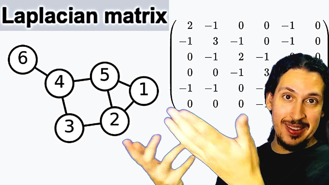
The graph Laplacian is defined as L = D - A, where D is the degree matrix (diagonal matrix containing node degrees) and A is the adjacency matrix (binary matrix indicating node connections); it possesses key properties including row/column sums equaling zero, non-negative real eigenvalues, and orthogonal eigenvectors, making it fundamental for spectral graph analysis.
Defining the Graph Laplacian: Advanced Lecture 32
Added:Basic graph theory concepts, including vertices, edges, node degrees, and the difference between directed and undirected graphs.

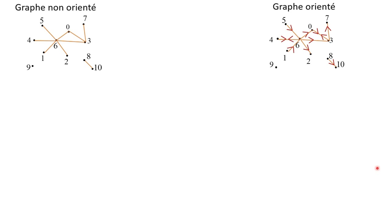
A graph consists of vertices (nodes) and edges connecting them. The number of vertices is called the order of the graph. Graphs are classified as undirected (edges traversable in both directions) or directed (edges traversable in one direction, called arcs). Adjacency describes when two vertices are connected by an edge. In undirected graphs, adjacency is symmetric; in directed graphs, it is directional. The degree of a vertex in an undirected graph equals the number of incident edges (or neighbors). In directed graphs, we distinguish out-degree (edges originating from the vertex) and in-degree (edges arriving at the vertex). A fundamental property: the sum of all vertex degrees in an undirected graph equals twice the number of edges, since each edge contributes to two vertices' degrees.

Graph theory studies diagrams composed of vertices (points) connected by edges (lines or curves). A graph is denoted as G = (V, E), where V represents vertices and E represents edges. Two fundamental graph types exist: directed graphs with arrowed edges specifying direction (having initial and terminal vertices), and undirected graphs without arrows. Key vertex properties include adjacency (vertices sharing a direct connection), loops (edges connecting a vertex to itself), and isolated vertices (unconnected vertices). Parallel edges share identical initial and terminal vertices. Graphs are classified as simple graphs (no loops or parallel edges), general graphs (at least one loop or parallel edge), complete graphs (every vertex connected to every other), and weighted graphs (edges assigned real number weights). Degree measurement differs between directed and undirected graphs: undirected graphs have total degree (edges incident to the vertex), while directed graphs distinguish in-degree (incoming edges) and out-degree (outgoing edges), with total degree being their sum.

A graph G = (V, E) consists of a non-empty set of vertices V and a set of edges E, where each edge connects one or two vertices (endpoints). Graphs are classified as: undirected (no direction on edges) or directed (edges have direction represented as ordered pairs); simple (no multiple edges or loops), multigraph (multiple edges allowed but no loops), or pseudograph (both multiple edges and loops allowed). Key concepts include adjacent vertices (connected by an edge), neighborhood (set of adjacent vertices), and degree (number of incident edges, with loops counting twice). The Handshaking Theorem states that the sum of all vertex degrees equals twice the number of edges. For directed graphs, in-degree (edges entering a vertex) and out-degree (edges leaving a vertex) are defined, with loops contributing to both. The sum of in-degrees equals the sum of out-degrees, which equals the total number of edges.

A graph is a mathematical structure consisting of vertices (points/nodes) and edges (lines connecting vertices). Key concepts include: loops (edges connecting a vertex to itself), pendant vertices (degree 1), isolated vertices (degree 0), adjacency (vertices connected by an edge), parallel edges (multiple edges between same vertices), multigraphs (graphs with parallel edges), order (number of vertices), size (number of edges), directed vs undirected graphs, simple graphs (no loops or parallel edges), pseudographs (allow loops and parallel edges), degree of a vertex (number of incident edges), in-degree and out-degree (for directed graphs), and degree sequence (list of vertex degrees in ascending/descending order).

A graph consists of vertices (V) and edges (E), where edges connect one or two vertices (endpoints). Loops have only one endpoint. Graph pictures can be misleading—only edge connections matter, not geometry. Simple graphs have no loops or multiple edges between vertices. Two basic types exist: undirected graphs (edges have no direction) and directed graphs (edges have direction as ordered pairs). Key terminology includes: edges incident to vertices, adjacent/neighbor vertices, degree (number of incident edges, loops count as 2), in-degree (edges entering a vertex), and out-degree (edges leaving a vertex).
Matrix representations of graphs, specifically how to construct and interpret Adjacency Matrices and Degree Matrices.

An adjacency matrix is a table that records direct links between graph vertices. To construct it: list vertices as row and column headings, then fill cells with link counts. Loops count as two links. The matrix is symmetrical for undirected graphs. For example, with vertices A-G, you record one link between A-B, two links between E-F, and so on. This representation is essential for algorithms like Prim's algorithm.

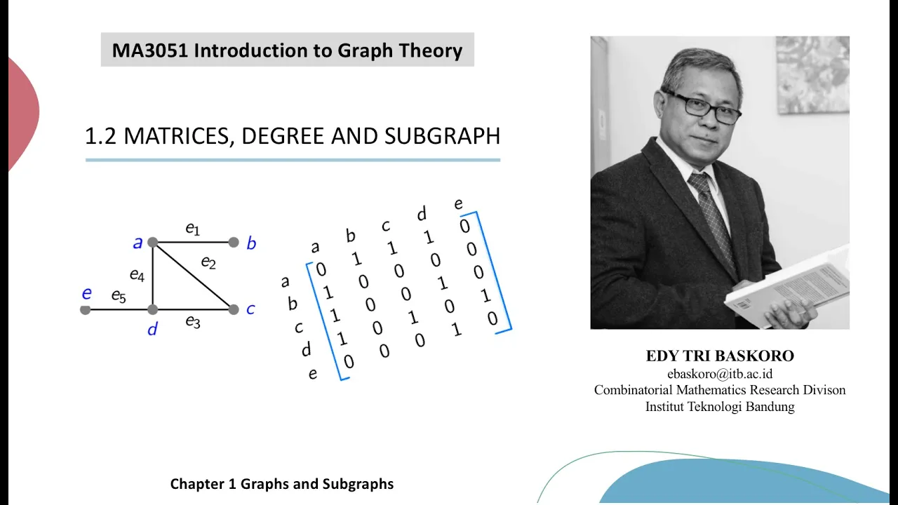
This section covers two fundamental matrix representations of graphs. The incidence matrix (N×M) represents vertex-edge relationships with entries of 1 when a vertex is an endpoint of an edge, and 0 otherwise. Each column contains exactly two 1s for simple graphs, and row sums equal vertex degrees. The adjacency matrix (N×N) represents vertex connectivity with entries of 1 when vertices are adjacent. For simple undirected graphs, diagonal entries are 0 and the matrix is symmetric. Key properties include: pendant vertices have rows with single 1s, isolated vertices have rows of all 0s, and disconnected graphs produce block diagonal matrices. These matrices provide algebraic frameworks for analyzing graph structure.

Graphs can be represented using matrices: (1) Adjacency matrix (square, symmetric for undirected graphs) where entry (i,j) equals the number of edges from vertex i to vertex j; (2) Incidence matrix (rows=vertices, columns=edges) where entry Aij=1 if vertex i is incident to edge j; (3) Circuit matrix (rows=circuits, columns=edges) where entry Aij=1 if edge j belongs to circuit i. The video demonstrates constructing these matrices for sample graphs and calculating vertex degrees from matrix entries.

Graphs can be represented using two types of matrices: Incidence Matrix and Adjacency Matrix. The Incidence Matrix has rows representing vertices and columns representing edges (n × m dimensions), with element a_ij = 1 if edge j is incident on vertex i. Key properties: each column has exactly two 1s, zero rows indicate isolated vertices, identical columns indicate parallel edges, and row sums equal vertex degrees. The Adjacency Matrix is square (n × n) with both rows and columns representing vertices, with element a_ij = 1 if edge exists between vertices i and j. Properties: diagonal elements indicate self-loops, row sums equal vertex degrees. For directed graphs, incidence matrices use +1 for outgoing edges and -1 for incoming edges.

A graph is completely determined by its adjacencies or incidences, which can be represented in matrix form. The adjacency matrix is an n×n matrix where entry a_ij represents the number of edges between vertices i and j (1 for simple graphs if adjacent). The incidence matrix is an n×m matrix where entry m_ij represents how many times vertex i and edge j are incident (0, 1, or 2 for loops). Row/column sums in the adjacency matrix give vertex degrees, and the matrix is always symmetric. Each column in the incidence matrix has exactly two 1s, representing that each edge connects two vertices.
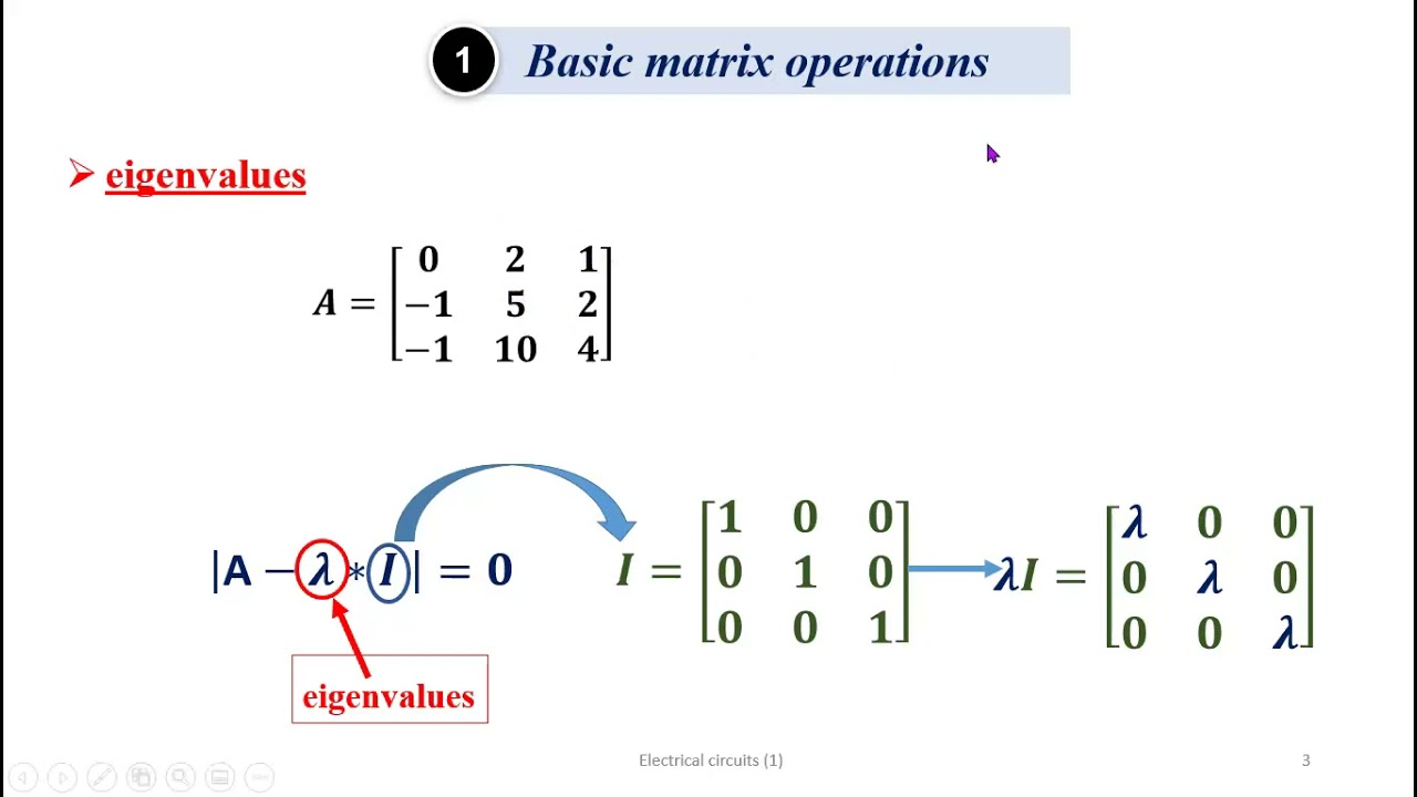
Fundamental linear algebra, including matrix subtraction, symmetric matrices, and the calculation of eigenvalues and eigenvectors.

Matrix subtraction is performed element-wise by subtracting corresponding elements from two matrices of the same dimensions. The process involves writing matrix A, adding the minus sign, then writing matrix B, and calculating the difference of each corresponding pair. For example, if A = [1 2; 3 4] and B = [5 6; 7 8], then A - B = [-4 -4; -4 -4]. When subtracting matrices with negative values, the same rule applies, and subtracting a negative number becomes addition.

The difference of two symmetric matrices is also symmetric. The instructor demonstrates this property by showing how subtracting two symmetric matrices results in another symmetric matrix.

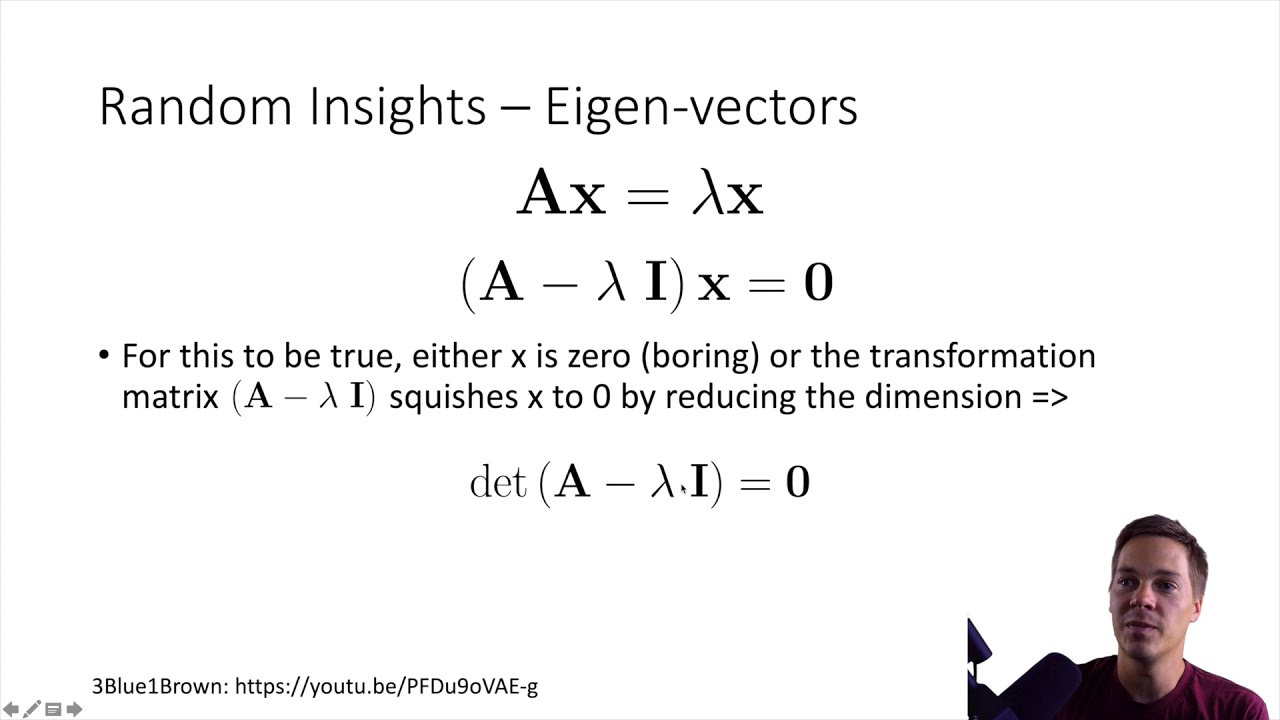
Matrix addition/subtraction requires identical dimensions. Eigenvalues are calculated using eig() function, which solves the characteristic equation det(A - λI) = 0. The result is a vector of eigenvalues representing the roots of the characteristic polynomial.

The video demonstrates the process of subtracting a scalar multiple of the identity matrix from a given matrix. When lambda equals 1, the instructor shows how to compute (A - I) by subtracting 1 from each diagonal element of the matrix. This results in a new matrix where the diagonal elements become zero, which is then used to solve for the eigenvector by setting the resulting matrix times the eigenvector equal to zero.

To compute A - K·I, multiply the identity matrix by K, then subtract this result from matrix A element-wise. For example, if A = [[-1, -2, -3], [4, 5, -6], [7, -8, 9]] and K = 5, then A - 5I = [[-1-5, -2-0, -3-0], [4-0, 5-5, -6-0], [7-0, -8-0, 9-5]] = [[-6, -2, -3], [4, 0, -6], [7, -8, 4]].
The concept of positive semi-definiteness and the Spectral Theorem for symmetric matrices.

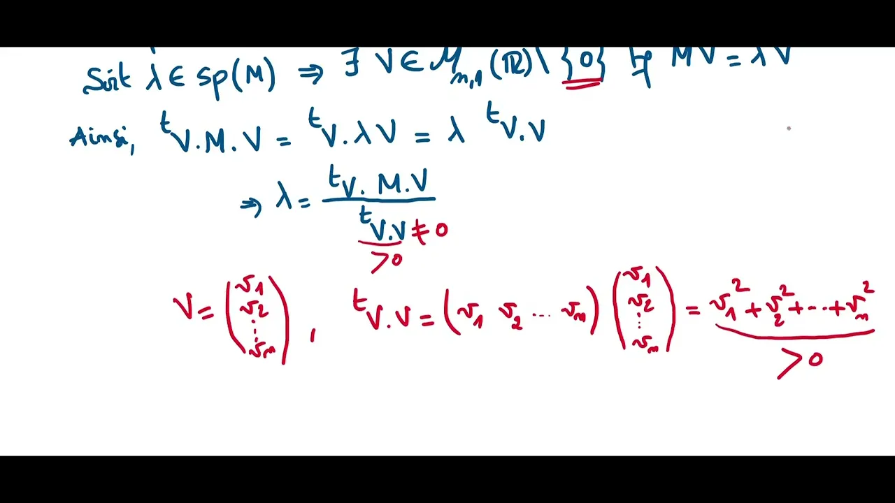
A matrix M is positive semi-definite if x* M x ≥ 0 for all vectors x, and positive definite if x* M x > 0 for all non-zero x. A key result is that a matrix is positive semi-definite if and only if all its eigenvalues are non-negative, and positive definite if and only if all eigenvalues are strictly positive. The spectral theorem states that real symmetric matrices are diagonalizable over the reals, which is fundamental to understanding positive matrices. For symmetric matrices, any eigenvalue must be real, proven by computing x* M x in two ways: as λ x* x and as λ̄ x* x, showing λ = λ̄.

If a symmetric matrix M has all strictly positive eigenvalues, then M is positive definite. Proof: By the Spectral Theorem, M = P D P^T where D = diag(λ₁, ..., λₙ) with λᵢ > 0. For any non-zero vector x, let y = P^T x. Then x^T M x = y^T D y = Σ λᵢ yᵢ². Since λᵢ > 0 and x ≠ 0 implies y ≠ 0, at least one yᵢ ≠ 0, so the sum is strictly positive. Thus M is positive definite.

Real symmetric matrices (A^T = A, real entries) have the fundamental property of spectral decomposition: A = QΛQ^T, where Λ is diagonal with real eigenvalues and Q is unitary (Q^T Q = I). The columns of Q are orthogonal and normalized. A symmetric matrix is positive semi-definite (PSD) if x^T A x ≥ 0 for all x, and positive definite (PD) if x^T A x > 0 for all non-zero x. Equivalent conditions for PSD: all eigenvalues ≥ 0, all principal minors ≥ 0, or A = B^T B for some B. For PD, B is square and non-singular. These concepts are essential for understanding convex optimization and semidefinite programming.

A symmetric matrix X is positive semi-definite (X ∈ S⁺ⁿ) if for all vectors z, zᵀXz ≥ 0. Equivalently, all eigenvalues of X are non-negative. For a 2×2 matrix [[a, b], [b, c]], this requires a ≥ 0, c ≥ 0, and ac - b² ≥ 0 (determinant condition).

A symmetric matrix S is positive semi-definite if x^T S x ≥ 0 for all non-zero vectors x. This allows the quadratic form to equal zero even when x ≠ 0, resulting in an infinite number of minimum points (like a taco shape). The eigenvalue condition is that all eigenvalues are greater than or equal to zero. Unlike positive definite matrices, positive semi-definite matrices are generally not invertible unless they are also positive definite (with no zero eigenvalues).
Prerequisite Knowledge
- Concept 01Basic graph theory concepts, including vertices, edges, node degrees, and the difference between directed and undirected graphs.
- Concept 02Matrix representations of graphs, specifically how to construct and interpret Adjacency Matrices and Degree Matrices.
- Concept 03Fundamental linear algebra, including matrix subtraction, symmetric matrices, and the calculation of eigenvalues and eigenvectors.
- Concept 04The concept of positive semi-definiteness and the Spectral Theorem for symmetric matrices.
Subsequent Learning
- Step 01Spectral Clustering, focusing on how the Fiedler vector (the eigenvector corresponding to the second smallest eigenvalue) is used for graph partitioning.
- Step 02The Normalized Graph Laplacian (both symmetric and random-walk normalized forms) and its advantages in spectral analysis.
- Step 03Diffusion processes on graphs, including how the Laplacian matrix is used to model random walks and the heat equation on networks.
- Step 04Introduction to Graph Convolutional Networks (GCNs) and how spectral graph theory underpins modern geometric deep learning.
- Step 05Kirchhoff's Matrix Tree Theorem, which uses the determinant of the Laplacian's cofactors to count the number of spanning trees in a graph.
Graph Matrices
0:00- 1
Defines adjacency and degree matrices for graphs.
- 2
Introduces the graph Laplacian as degree minus adjacency.
The Non-Backtracking Matrix and Laplacian Localization in Sparse Graphs
While the standard Graph Laplacian is a foundational tool in spectral graph theory, it suffers from severe limitations when applied to sparse, heterogeneous, or scale-free networks—structures common in real-world data. In these networks, the leading eigenvectors of the standard and normalized Laplacians tend to 'localize' around high-degree hub nodes rather than reflecting the global community structure. This localization bottleneck prevents effective spectral clustering and partitioning. To overcome this, researchers introduce alternative operators like the Non-Backtracking (or Hashimoto) Matrix. Unlike the Laplacian, which is defined on nodes, the non-backtracking matrix operates on directed edges and prevents trivial self-returning paths. This spectral alternative successfully detects communities down to the theoretical 'detectability threshold' where Laplacian-based methods fail completely. Thus, the non-backtracking perspective challenges the supremacy of the standard Laplacian in sparse network analysis, offering a more robust mathematical framework for real-world graph partitioning.
Spectral Clustering, focusing on how the Fiedler vector (the eigenvector corresponding to the second smallest eigenvalue) is used for graph partitioning.

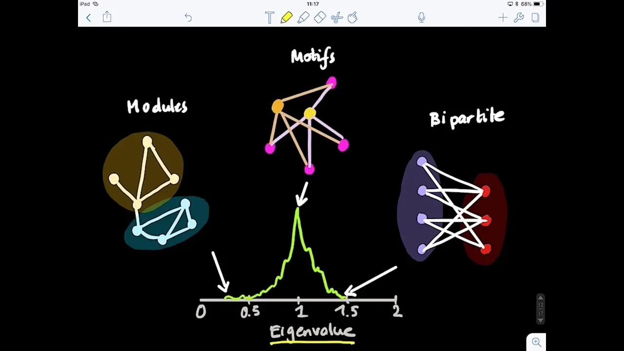
Spectral graph theory studies the eigenvalues and eigenvectors of graph matrices (particularly the Laplacian matrix L = D - A, where D is the degree matrix and A is the adjacency matrix) to analyze graph properties; the Laplacian matrix is called so because it measures the discrepancy between a vertex's value and the average of its neighbors, similar to the continuous Laplacian operator, and its second smallest eigenvalue (the Fiedler value) and corresponding eigenvector (the Fiedler vector) reveal natural partitions or communities within a graph, making spectral embedding and spectral clustering powerful tools for graph partitioning and machine learning applications.

The second smallest eigenvalue (λ₂) and its corresponding eigenvector (Fiedler vector) of the graph Laplacian matrix provide an optimal solution for graph bisection, where the eigenvector assigns real-valued labels to nodes such that the sum of squared differences across all edges is minimized, effectively identifying two clusters with minimal edge cuts between them.

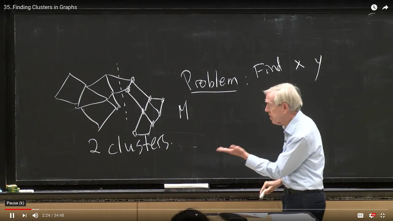
Spectral clustering is a graph clustering technique that uses the eigenvalues and eigenvectors of the graph Laplacian matrix to identify clusters. The graph Laplacian L = D - A (where D is the degree matrix and A is the adjacency matrix) is a symmetric positive semi-definite matrix whose smallest non-zero eigenvalue (called the algebraic connectivity) and its corresponding eigenvector (called the Fiedler vector) reveal the natural partitions in a graph. The Fiedler vector has positive and negative components, and nodes are assigned to different clusters based on the sign of their corresponding component in this eigenvector. This method provides a powerful alternative to iterative algorithms like K-means for finding meaningful clusters in complex networks.

The min-cut problem seeks to partition graphs by minimizing cross-cluster edges. Relaxing binary cluster assignments to real values leads to optimizing x^T L x, which equals twice the number of cross-cut edges. Constraints ensure meaningful solutions: center-of-mass at origin prevents trivial constant mappings, and normalization ensures non-zero vectors. The Rayleigh-Ritz theorem shows the optimal solution is the eigenvector with the second-smallest eigenvalue—the Fiedler vector—which provides one-dimensional cluster embeddings.

The Fiedler vector, which is the second smallest eigenvector of a graph's Laplacian matrix, enables binary clustering by providing a zero-mean signal that partitions vertices into two groups based on the signs of its entries; since the Laplacian matrix is symmetric positive semi-definite with a guaranteed zero eigenvalue corresponding to the ones vector, the Fiedler vector is orthogonal to this trivial eigenvector and serves as the fundamental tool for spectral clustering algorithms.
The Normalized Graph Laplacian (both symmetric and random-walk normalized forms) and its advantages in spectral analysis.

The normalized Laplacian is defined as I - D^{-1/2}AD^{-1/2}, which is similar to the transition probability matrix P = D^{-1}A for random walks on graphs. In a random walk, at each step you move uniformly to a random neighbor. The normalized Laplacian is similar to the symmetric matrix D^{-1/2}LD^{-1/2} = I - D^{-1/2}AD^{-1/2}, so they share the same eigenvalues. These eigenvalues control the mixing time of random walks, determining how quickly the walk converges to its stationary distribution.

The normalized Laplacian is defined as D^(-1/2)LD^(-1/2), where D is the diagonal matrix of vertex degrees. For a k-regular graph, this simplifies to I - (1/k)A, where A is the adjacency matrix. This normalization ensures that the Laplacian becomes a symmetric matrix, which is important for spectral analysis and has connections to random walk theory.

Two approaches define graph convolution: spectral (using Laplacian eigenvectors/eigenvalues) and spatial (localized averaging). The graph Laplacian measures signal variation at each vertex relative to neighbors. For cycle graphs, it corresponds to the discrete second derivative. Multiple Laplacian variants exist: normalized, symmetric normalized, and random walk versions. These symmetric matrices enable straightforward spectral analysis, with eigenvectors forming natural Fourier bases for harmonic analysis on graphs.

The normalized Laplacian L̃ = D^(-1/2)LD^(-1/2) = I - D^(-1/2)AD^(-1/2) scales the standard Laplacian so eigenvalues lie in [0,2]. This normalization preserves symmetry and connects directly to random walks: P = D^(-1)A is similar to I - L̃, sharing the same eigenvalues. The smoothing property of the Laplacian—subtracting neighbor averages from node values—makes it valuable for applications including image denoising and regression on graphs. By running diffusion for limited iterations, noise can be removed while preserving image structure. The normalized Laplacian also provides theoretical guarantees for graph partition quality through Cheeger-type inequalities relating eigenvalues to conductance measures.

The normalized Laplacian divides each element by the starting node's strength, creating a probability transition matrix where diagonals equal 1. This enables direct comparison of node importance and facilitates random walk analysis. For symmetry, divide each element by √(S_i × S_j), ensuring the matrix is self-adjoint. These normalized forms preserve essential structural information while enabling standardized comparison across different network scales and configurations.
Diffusion processes on graphs, including how the Laplacian matrix is used to model random walks and the heat equation on networks.

The Laplacian matrix (L = D - A) has rows that sum to zero. It emerges naturally from diffusion processes (heat/chemical spreading) and random walks (personalized PageRank). The structure D - A appears repeatedly in graph algorithms because it enables elegant mathematical formulations of diffusion and random walk dynamics.

Random walks on graphs are stochastic processes where a walker moves from node to node with transition probabilities proportional to node degrees, eventually converging to a stationary distribution proportional to node degrees; diffusion on graphs can be modeled using the discrete Laplace operator (Laplacian matrix L = D - A), where the long-term behavior is determined by the eigenvalues and eigenvectors of this matrix, with the second smallest eigenvalue (Fiedler value) and its corresponding eigenvector (Fiedler vector) being particularly important for understanding how quantities spread across the graph and for spectral graph partitioning.

The Laplacian matrix has non-negative eigenvalues with zero multiplicity equal to connected components. The matrix tree theorem gives spanning tree count as product of non-zero eigenvalues divided by n. The probability transition matrix governs random walks, with real eigenvalues for connected non-bipartite graphs. Convergence to stationary distribution depends exponentially on eigenvalue gaps—values near 1 cause slow mixing while values near 0 enable rapid convergence. This connects spectral analysis to diffusion processes on networks.

The graph Laplacian is a symmetric matrix defined by the quadratic form that sums weighted squared differences across edges, and it serves as a fundamental tool connecting various linear algebraic processes on graphs including random walks (where probabilities evolve as P = D⁻¹A), heat diffusion (governed by the heat equation ∂u/∂t = -Lu), and electrical networks (where currents minimize energy subject to Kirchhoff's laws), with its spectral properties revealing key structural information about the graph such as the number of connected components (equal to the multiplicity of zero eigenvalues) and bounds on eigenvalues related to the maximum degree.

Diffusion processes on networks can be modeled using the Laplacian matrix through the governing equation dX/dt = -LX, where X is a vector representing the state of each node (such as the number of random walkers at each node). The solution involves expanding the initial condition in terms of the Laplacian's eigenvectors: X(t) = Σ c_i e^(-μ_i t) v_i. The stationary state is determined by the zero eigenvalue (μ₀ = 0), while the mixing time or diffusion time scale is determined by the second smallest eigenvalue μ₁, specifically T_diffusion ≈ 1/μ₁. This shows how spectral properties directly control both the equilibrium behavior and the approach to equilibrium in network dynamics.
Introduction to Graph Convolutional Networks (GCNs) and how spectral graph theory underpins modern geometric deep learning.

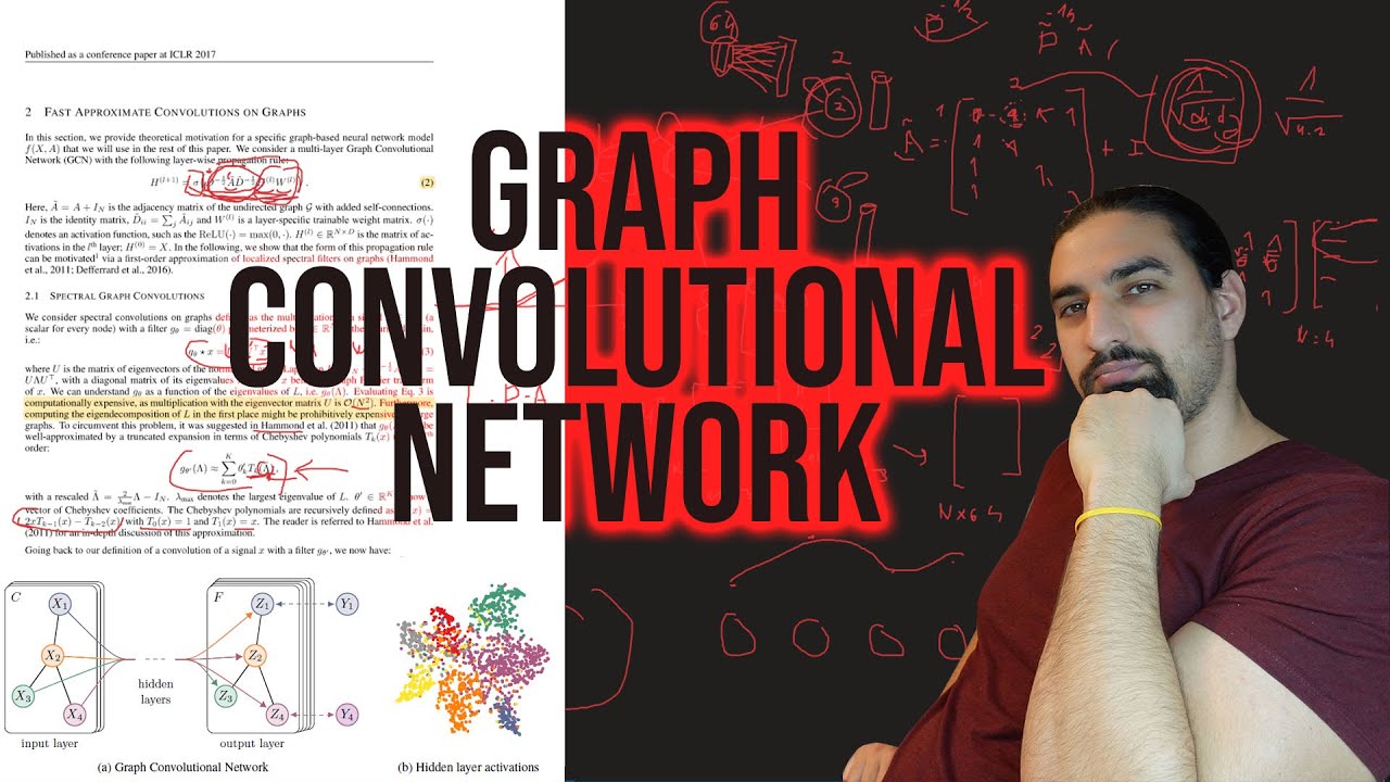
Graph Convolutional Networks (GCN), introduced by Thomas Kipf and Max Welling, are semi-supervised learning models that propagate node features through normalized adjacency matrices (D̃^(-1/2) Ã D̃^(-1/2)) to aggregate information from neighboring nodes, achieving state-of-the-art performance on citation networks by learning to smooth labels across connected nodes; GCN can be understood through three perspectives: as a spectral method approximating Chebyshev polynomial filters on graph Laplacians with k=1, as a generalized Weisfeiler-Lehman algorithm with differentiable aggregation, and as a specific case of message-passing neural networks, though it has limitations in distinguishing certain graph structures compared to more expressive variants like GIN.

Graph Convolutional Networks (GCNs) extend traditional neural networks by leveraging graph structure. The core concept is message passing: nodes send information to neighbors and collect messages to update their own state. Unlike label propagation which only smooths labels, GCNs perform feature smoothing by processing entire attribute vectors. A single GCN layer works by first aggregating neighbor attribute vectors (e.g., averaging) and then passing this aggregated vector through a dense neural network layer using matrix multiplication and activation functions. This two-step process—aggregate then transform—forms the fundamental building block of GCNs.

Graph Convolutional Networks (GCNs) are neural network models designed to process graph-structured data by performing convolutions over nodes and their neighbors; the model aggregates information from a node's immediate neighborhood using the adjacency matrix, normalizes the aggregation by dividing by the square root of the product of node degrees (D^(-1/2)AD^(-1/2)), incorporates self-loops by adding an identity matrix to the adjacency matrix, applies learnable weight matrices, and passes the result through non-linear activation functions to transform node features from D dimensions to D' dimensions.

Graph Convolutional Networks (GCNs) extend traditional convolutional neural networks to handle irregular graph-structured data by defining two main approaches: (1) Spectral GCNs use graph Fourier transforms and Chebyshev polynomials to achieve linear complexity O(k·|E|) for sparse graphs, enabling efficient learning of localized spatial filters; (2) Spatial GCNs use template matching with attention mechanisms to create anisotropic filters that adaptively weigh neighboring nodes based on their properties, achieving O(|E|) complexity. Both approaches enable powerful feature extraction for diverse applications including social networks, brain connectivity analysis, molecular property prediction, and recommendation systems.

Spectral graph theory studies the eigenvalues and eigenvectors of graph matrices (particularly the Laplacian matrix L = D - A, where D is the degree matrix and A is the adjacency matrix) to analyze graph properties; the Laplacian matrix is called so because it measures the discrepancy between a vertex's value and the average of its neighbors, similar to the continuous Laplacian operator, and its second smallest eigenvalue (the Fiedler value) and corresponding eigenvector (the Fiedler vector) reveal natural partitions or communities within a graph, making spectral embedding and spectral clustering powerful tools for graph partitioning and machine learning applications.
Kirchhoff's Matrix Tree Theorem, which uses the determinant of the Laplacian's cofactors to count the number of spanning trees in a graph.

To find the number of spanning trees using Kirchhoff's theorem, compute the cofactor of any element in the Kirchhoff matrix. The cofactor is calculated by: (1) Removing the row and column containing the chosen element, (2) Computing the determinant of the resulting submatrix, (3) Applying alternating signs (+, -, +, ...) based on the position. The resulting value equals the number of spanning trees in the graph. For example, a graph might have 8 spanning trees.

Kirchhoff's Matrix Tree Theorem counts spanning trees: (1) Create adjacency matrix with 1s for edges, (2) Replace diagonal with vertex degrees, (3) Replace non-diagonal 1s with -1, (4) Find any cofactor. For complete graph K_n, the formula is n^(n-2). For example, K_4 has 4^(4-2) = 16 spanning trees. The cofactor calculation yields the exact number of spanning trees for any graph.

This comprehensive section covers the mathematical foundations and complete proof of Kirchhoff's Matrix-Tree Theorem. It begins with cofactor and adjugate matrix definitions, establishing that M × adj(M) = det(M) × J and M⁻¹ = adj(M)/det(M) when det(M) ≠ 0. The theorem states that for any graph Γ with Laplacian L, adj(L) = τ(Γ) × J, where τ(Γ) is the number of spanning trees. The proof uses case analysis: disconnected graphs have rank ≤ n-2, forcing adj(L) = 0; connected graphs have rank n-1, yielding adj(L) = αJ with α ≠ 0. The critical step applies the Binet-Cauchy formula to show that det(L_x) counts spanning trees, as only spanning tree edge sets contribute non-zero terms. Two equivalent formulas are derived: τ(Γ) = det(J + L)/n² and τ(Γ) = (μ₂ × μ₃ × ... × μₙ)/n, connecting combinatorial graph properties to algebraic invariants.

This comprehensive section develops the Matrix Tree Theorem (Kirchhoff's Theorem), which states that any algebraic complement of the Laplacian matrix equals the number of spanning trees in the graph. The Laplacian matrix L is defined as L = B × B^T, where B is the incidence matrix. Key properties include: multiplying a row of B by itself yields the vertex degree, while multiplying different rows yields -1 if an edge exists between corresponding vertices. For graphs with n vertices and n-1 edges, the principal minor of B equals +1 or -1 if and only if the graph is a tree. The Binet-Cauchy formula enables computing determinants of matrix products as sums of submatrix determinants. Applying this to L = B × B^T, each term corresponds to a subgraph with n-1 edges, with determinant +1 or -1 if it's a tree and 0 otherwise. Thus, the sum equals the number of spanning trees.

The Laplacian matrix of a graph, constructed by placing node degrees on the diagonal and -1 for each edge between nodes, has a key property: the determinant of any cofactor (obtained by removing any row i and column i) equals the number of spanning trees in the graph. This works because when the Laplacian matrix is expanded algebraically with variables representing edges, each monomial in the determinant corresponds to exactly one spanning tree, and substituting 1 for existing edges and 0 for non-existing edges counts only valid spanning trees. The algorithm runs in O(n³) time using determinant computation.
Graph Matrices
0:00- 1
Defines adjacency and degree matrices for graphs.
- 2
Introduces the graph Laplacian as degree minus adjacency.
The Non-Backtracking Matrix and Laplacian Localization in Sparse Graphs
While the standard Graph Laplacian is a foundational tool in spectral graph theory, it suffers from severe limitations when applied to sparse, heterogeneous, or scale-free networks—structures common in real-world data. In these networks, the leading eigenvectors of the standard and normalized Laplacians tend to 'localize' around high-degree hub nodes rather than reflecting the global community structure. This localization bottleneck prevents effective spectral clustering and partitioning. To overcome this, researchers introduce alternative operators like the Non-Backtracking (or Hashimoto) Matrix. Unlike the Laplacian, which is defined on nodes, the non-backtracking matrix operates on directed edges and prevents trivial self-returning paths. This spectral alternative successfully detects communities down to the theoretical 'detectability threshold' where Laplacian-based methods fail completely. Thus, the non-backtracking perspective challenges the supremacy of the standard Laplacian in sparse network analysis, offering a more robust mathematical framework for real-world graph partitioning.
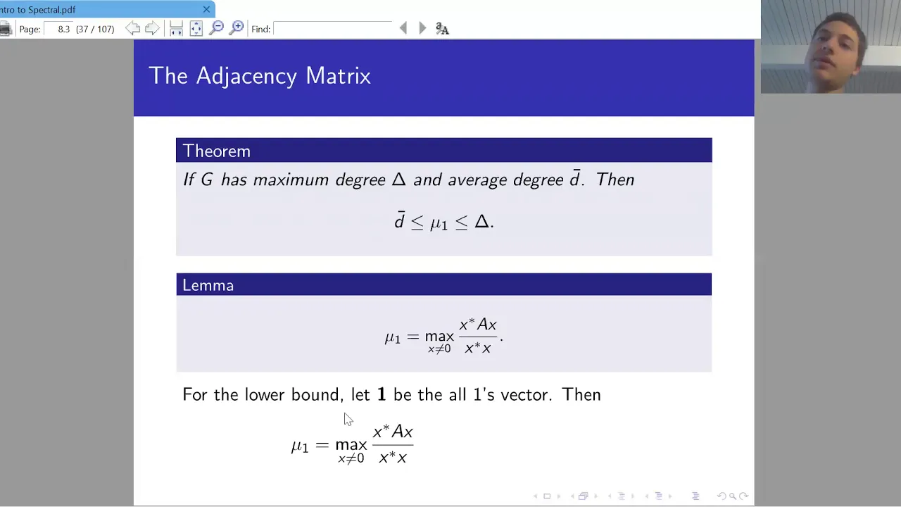
so now let's start building on this intuition and let's start thinking about what is the right graph uh Matrix representation that will allow us to use this intuition from the previous slide right so we have already defined the graph adjacency Matrix which is an N byn Matrix where n is the number of nodes and we simply say that AI J equals 1 if node I links to node J and otherwise it has value zero so for a given graph G here this is the adjacency Matrix a which is a binary adjacency Matrix where um value of one means that a g pair of nodes is connected and zero means it doesn't uh what are some properties of this um of the spectrum or the IG values and igen vectors of this adjacent symatrix uh first this is a symmetric Matrix right because our graph is undirected and because of that igen vectors um of our adjacency Matrix are real so are real valued and they are orthogonal by definition and these are the two important properties that we will exploit later so this is now the definition of the adjacency Matrix let's also Define what we will call a degree Matrix d right so for a G given graph G an degree Matrix D is simply a diagonal matrix where for a given diagonal entry the value there is simply the degree of a given node right so for example in our case node number one has three uh a edges adjacent to it which basically means that here um in the entry one one of our uh degree Matrix we have an entry three this is now the definition of the degree Matrix so now what we are ready to Define is to define the graph laian Matrix and this is simply an N byn Matrix where what we basically do is we take we label this Matrix as L and L is simply the degree Min degree Matrix minus the adjacency Matrix right so now I have a matrix where on the diagonal I have the degrees of the nodes and of the of the diagonal I have binary entries either Z or minus one zero means that a given pair of entries of nodes is not connected and minus one means that a pair of nodes is connected what are some properties of this Matrix for example one property that we notice is that the sum of entries in every row equals to zero right because the number of minus ones that we have in every every row is exactly the degree of the node and on the diagonal we have the positive degree of that node so the two things cancel out so each row and each column of this Matrix sums to uh zero what this basically means is that we have already found a trivial igen pair right so if we have a vector X of all values of um one then if you ask okay I a * X is simply the sum of the labels of my of my neighbors all my neighbors have entry minus one so I get minus D on the diagonal I have an entry D so basically it means that L * x equals 0 which means that Lambda 1 so the smallest igen value of this uh adjacency Matrix uh equals uh zero and then what are other important properties of this uh laian Matrix first is that IG values are non- negative real valued numbers and the second one is again that igen vectors are real and orthogonal orthogonal means that when I do a DOT product of two ve igen vectors their dot product is zero
Up Next

Markov Chains Explained: From Russian Feud to Modern Algorithms
@veritasium
10.6M views•2025-07-25

Gain Recalibration in Hippocampal Path Integration: Math Theory
@1024kyz
144 views•2020-07-02

Fourier Series Introduction: The Big Idea Explained
@DrTrefor
387K views•2021-05-03

The Mathematical Impossibility of Accurate World Maps
@Vox
23.3M views•2016-12-02
Related Study Plans & Knowledge Roadmaps
Structured learning paths in Mathematics
