Spectral Graph Theory Explained: Laplacian, Eigenvalues, and Clustering

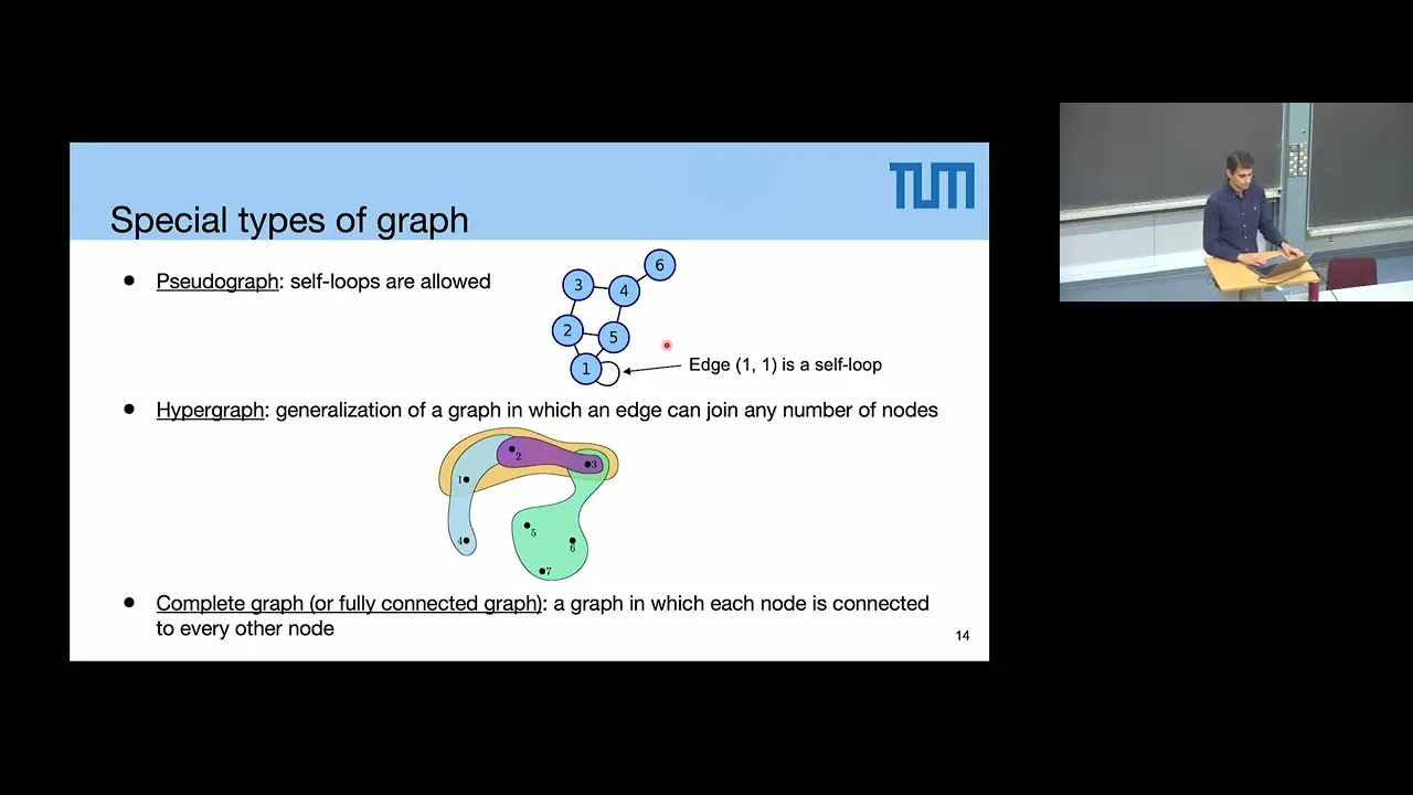
[00:00:00]brilliant sponsored this video more brilliant later yes yes you heard me right a graph does have AG values the study of a graphs property using linear algebra is called spectrograph Theory this field of study is huge and fascinating but the most fundamental idea of spectrograph theory is simple and beautiful easy to understand let's take a look shall we here is the after of this video we will talk about some basic graph Theory then we will do a review of linear algebra next we talk about the graph laash and some of its basic properties then we move on to the fedal value and the fedal vector at the end we talk about probably the most famous application of spectr graph theory in machine learning spectr clasy now let's get started a graph G is made of vertices and edges the collection of vertices is denoted as V and the collection of edges is denoted as e for example this graph has five vertices denoted as V1 up to V5 and it has six edges denoted as tle or topos of VI VJ for example V1 V2 means there's Edge between vertex one and Vortex 2 generally speaking the edges can have directions it's just like on social Network I follow you on Instagram but you may not follow me back in this video we make the assumption that the edges are undirectional it's like a genuine friendship I'm your friend then you are my friend the graph is also called undirected graph the degree of a Vertex is the number of neighbors or connections of the vertex the vertex with the highest degree is like the most popular guy in your social bubble suppose I remove two edges from this graph I'm intuitively decreasing the level of connectivity of this graph but if you look at this graph and the original graph they have something in common they're both connected a graph is connected means that I can start from any vertex of the graph and reach any other vertex following a sequence of edges intuitively the more connected the graph is the shorter the path may be removing one more Edge there's no way to start from Vortex 5 to reach Vortex 2 we say this newr is disconnected but it has two connected components all right let's quickly exam some typical graphs degrees the Accel vertices form a valid graph but the degrees are all zero vertices of a line graph has degrees of two except those two vertices at the end the cycle graph is highly symmetric it has equal degrees for everyone an opposite extreme example is a star graph it has a high level of imbalance of degree a complete graph a fully connected graph is like a Utopia of degrees if there are n vertices then each vertex has the highest possible of degree n minus one for General disconnected graph usually there is no pattern to follow this graph is also a good example that we cannot reconstruct the graph using the degree information only for some special cases we can like this one and this one but not generally can you find another graph that has exactly the same degree information to capture all the connectivity information of a graph we need the adjacency Matrix a AIG J is defined as one if there is an edge between vertex V and vertex VJ take the first rowle as an example it means that vertex one is connected to vertex 2 Vertex 4 and Vex 5 because connection is mutal therefore the First Column is exactly the transpose of the first row if we sum each row of the adjacency Matrix and align them along the diagonal line we get the so-called degree Matrix a lot of information is lost during the summation process this agrees with our observations that you cannot use the degrees to construct the graph let's look at the adjacens matrices and the degree matrices of the graphs we mentioned earlier although those matrices look very different but they do share two characteristics in common first both matrices are symmetric which means the eal are transpose second all the entries are real numbers we call such matrices real symmetric matrices and they have some very nice properties for the disconnected graph with proper labeling we see a block structure in the adjacent Matrix this block structure has a big impact over the matrices igen value and igen vectors which which we will discuss deeply in a moment all right that's everything we need to know for the graph side of the spectral graph Theory now let's look at the spectral side spectral theory in general is a huge topic that spans across several fields of mathematics however if we focus on finite Dimension linear space Square matrices spectral Theory becomes a theory of ion value and ion vectors so what is spect graph Theory it is a study of aing values and aing vectors of graph matrices as we assume the graphs are all undirected so all the matrices associated with the graphs are real and symmetric real symmetric matrices are so good why first the real symmetric matrices are guaranteed to be diagnosable a matrix is diagonalizable means that we can find two Matrix p and Lambda such that the Matrix can can be written as P * Lambda * P inverse Lambda is a diagonal matrix here and for real symmetric Matrix the ion values are all real another great property of real symmetric Matrix is that the Symmetry is preserved under addition or subtraction for example D minus a gave us a new Matrix L it is called The laash Matrix we will talk about the laasia Matrix very shortly but now let's review three important properties of the ion values and ion vectors first zero is actually a valid ion value but zero Vector is not a valid ion Vector the highlighted ion Vector is the corresponding ion Vector for ION value zero it is essentially the solution to the homogeneous linear equations because the right hand side of the equation is essentially zero but an all zero eging Vector doesn't make any sense as the eging value can be any number the second important property is about orality Egon vectors of different Egon values are oral to each other here I'm using different colors to represent different pairs of EG value and Egon vectors two vectors being AAL means that their dot product is zero if you take any two EG vectors and find their dot product it is indeed zero the last important point to review is multiplicities the same Aon values may have different multiplicities for example in order to find the a values of these three matrices we solve the characteristic polinomial we find out that the first Matrix has two different values but the second and the third matrices have two as the only a value the terms that the a value appear as roots in the characteristic polom is called the algebraic multiplicity algebraic multiplicity is not the only Multiplicity taking a closer look at the second Matrix we see that the AG value two has two corresponding and orthogonal aen vectors it means the aen space spaned by the Egon vectors has a dimension of two the dimension of the Egen space of the Aon value is called the geometric multiplicity of the Egon value but when we try to find the two Egon vectors for the third Matrix we have trouble one Z is a valid Eon Vector but we cannot find the second Egen Vector that is orthogonal to 1 Z which means Egen space only has a dimension of one putting these examples together we see that the algebraic multiplicity is always greater than or equal to the geometric multiplicity Can you spot the difference between the first two matrices and the last one the first two matrices are both diagonalizable this is great news for our degree Matrix and adjacency Matrix because they are symmetric therefore they are always diagonalizable for the rest of the video I will just use the word multiplicity as we will limit our discussion to real symmetric matrices still remember the laan Matrix L equal D minus a the degree Matrix minus the adjacent symatrix The laion Matrix is a difference between two real symmetric Matrix so it is also real and symmetric there for all the nice properties we discussed earlier will also apply first let's see what will happen if we multiply a vector F we use f instead of V for two reasons the first reason is that I don't want to confuse you with V for Vertex or V for Vector second is that we will see the F Vector does have a meaning of a function that is defined on the graph let's check the I component of the new Vector LF we will see that it's actually the summation of the difference between fi and its neighbors again please please bear with me with a notation I'm writing fi and FJ as if f is a function instead of using the subscript I promise you that the reason will become clear later when I explain why the l Matrix is called The laash Matrix okay suppose f is eging Vector then we have LF = Lambda F therefore Lambda equal F transpose LF substitute the expression of LF we see a very interesting expression simplification by staring at it is not for normal people like you and me so let's expand it for this particular graph using the adjacency information the sumission can be grouped into four components simplifying one more step we see that the E value Lambda can be written as a summation of squares just by observing this result we can have a few important conclusions first L is positive semide definite it means all the eging values of L are non- negative second zero is always an aing value of L we can simply cting f as a constant the last observation is more hand waving for a given graph the smaller the Egon value is the smoother the Egon Vector is it is true because the smaller the difference between interest of the Egon vectors then the smaller the summation is on another hand if a vector happens to be eging vectors for two graphs then the one with a smaller Egon value is less connected because you have fewer terms to sum over now let's turn those intuitive observations into concrete examples for the isolated vertices because there's no connection at all therefore Lambda equals the summation of nothing therefore the only Egon value is zero and we can find four eging vectors that B the aen space of dimension of four our first non trival example is a l graph and we have four different Egon values for a better visual understanding let's plot those four Egon vectors and see how smooth they are as we mentioned earlier we can always pick a constant Vector as the Aon Vector of agon value zero and the first non constant Aon Vector has a smooth decreasing Trend you can verify it yourself if you consider the connectivity information in the graph the third and the fourth Egon vectors do have bigger and bigger variances now let's move on to the cyle graph the cycle graph clearly has a stronger Symmetry and this symmetry is reviewed in its Aon values and Aon vectors the agen value two has a multiplicity of two and it's two Egen vectors do look symmetric also look at the force Vector it is a vector that tries to maximize Aon value isn't it next let's move on to the star graph the star graph is the perfect example that when we interpret the Aon vectors we have to take the connectivity information into consideration for example why is the Aon Vector corresponding to the largest Aon value four is smoother or at least looks smoother than I Vector 2 and ion Vector 3 the reason that vortex one is at the center of the graph all we care about when we talk about the difference is the difference between vertex one and other vertexes and from this perspective I Vector 4 is the most rough one another good example that symmetry impacts the multiplicity of Icon values is a complete graph the complete graph only has two icon values zero and N where n is the number of vertices and the multiplicity of n is n minus one my intuitive way to make sense of this multiplicity is to think about the permutation we can verify that 311 1 is actually Anon Vector for the Aon value four and because of the Symmetry I can right shifted entries to get two more Egen vectors therefore the dimension of the Egen space is at least three but it's not four because the fource ion Vector will be linearly dependent on the first three therefore the multiplicity is three oh good now let's move on to our last example the graph with three connected components this one is particularly interesting because the Egon value zero has a multiplicity of three which is exactly the number of connected components look at the first ion Vector it seems that it's only non zero on the first connected component the same idea applies to the second and the third Anon Vector corresponding to the Aon value zero this is truly interesting and a more interesting question to ask is what information is hiding in the E vectors corresponding to other nonzero aen vectors to answer these questions it is beneficial to understand first why the l Matrix is called laash Matrix and what it does when we apply the L Matrix over a vector most likely you and me know this man laas for two reasons first the laas transform second the lapasan operator as we are not doing any integral so likely we need to focus on the lapas operator the laas operator calculates the Divergence of the gradient of a function incart cord it is the summation of the second partial derivatives for one dimensional case it is just the second derivative therefore for a linear function the laas of this function is zero everywhere imagine you are standing on this function at 0.5 0.5 you look at your neighbors in a small interval because the second derivative is zero the amount your right neighbor is higher than you is exactly the same amount that your left neighbor is lower than you but imagine a nonzero laas a negative second derivative means that you are higher than the average of your neighborhood you have much lower left neighbors than higher right neighbors and it becomes the opposite when the second derivative is positive the same idea applies to higher Dimensions we can construct a function whose laas is positive almost every from this angle it's very clear that the average function values in a small neighborhood is always larger than the value at the center the most naive understanding of the laas operator is that it measures the discrepancy between a function's value and the average of its neighborhood now you can understand why I use f instead of V to denote the E Vector imagine f is a function defined under vertices its neighborhood is restricted by the edges take vertex 2 as an example when we apply the laan Matrix on F the second entry of LF is essentially the sum of the differences between vertex 2 and its neighbors this is almost the laas operator if we find the average of it and of course there is the so-called normalized lashion Matrix which essentially divides each entry by the degrees we are not going to use the normalized laion in this video but you can convince yourself that it does exactly the same thing to a function defined on the graph as a lapas operator does to a normal function now let's look at our first agon value zero it turns out that the llas Matrix L has agon value zero with multiplicity K if and only if the graph has K connected components against some intuition let me bring back those examples again for the Accel vertices it's easier to sync about the multiplicity from the algebraic perspective therefore Zero's multiplicity is four for the CYO graph it's easier to think about it from the geometric perspective treat the AG Vector as a solution to the linear equations the four independent restrictions limit the dimension of the Egen space to be one let's prove it more rigorously first let's prove that the multiplicity of eon value zero is no less than the number of connected components we already see that with proper index we can find the block structure in the laash Matrix indexing is just assigning an order to the vertices we are free to index however we want so the block structure will always exist now we can construct Egon vectors whose corresponding entries of the block are nonzeros this this shows that if there are K connected components we can have at least K vectors of a value zero next let's prove the opposite using contradiction if there are K connected components because e value can be written as a sum of squares therefore it can be written as the sum of three sum of squares each of them has to be zero so we can construct K independent aen vectors just as before Suppose there is one more aen Vector because aen Vector cannot be zero therefore it must be non zero somewhere if one entry is non zero it is impossible to keep your neighbors zero therefore our extra Egon Vector cannot be linearly independent of our existing agon vectors which creates a contradiction sounds good let's move on to the second smallest Eon value to make left easier let's focus on the connected graphs recall that if the Egon values are different the corresponding Egon vectors are orthogonal here I'm using subscript to indicate that fub1 is Egon Vector corresponding to the first Eon value zero and F2 corresponds to the second ekon value a zero dot product suggests that the summation of Ines of F2 is zero but different from fub1 there will be up and downs in FS2 Lambda 2 and FS2 are called the fedler Egon value and fedler Egon Vector they are named after mathematician mirror SL fed H so why are Lambda 2 and F2 so important that they have their own names take a look at this graph let's calculate its faton value and faton Vector Lambda 2 is 0.36 and F2 is on the screen notice that the indexing is completely random therefore our L doesn't have a block structure but we will see that it doesn't change the nature of the graph it seems that the fedal vector finds a very nice paration of our original graph if we reconstruct the block structure the partitioning is more clear the feder vector finds a choke point the edge between Vortex 3 and Vortex 4 intuitively vertices 1 2 three form a community and vertices 4 5 6 7 form another and the edge 34 is the only connection between these two communities because Lambda 2 is non zero but it's also the smallest Egon value therefore F2 will behave like a pair of scissors it's going to find the weakest Connection in the graph and flip the signs of the interest of F2 there but this mechanism can easily break down for example why should I cut on this graph the Fatal Vector is not a solution to an artificial optimization problem just by the nature of a linear system the F Vector happens to do a reasonably good job when the graph is well behaved not this one we can fix it by dropping the weightless Edge assumption we can assum weights to different pairs of vertices to measure how close they are in real life this often break the Symmetry for example you must have one or two closest friends the new laash Matrix has a new definition but the core idea Remains the Same because vertex one is closer to vertexes 2 and three so this time this three will form a new community and the lashan Matrix also reveals a stronger Affinity between vertices 1 2 and three as we mentioned earlier the fular vector is not artificial but we can frame it as an optimization problem this direction naturally leads to the following question how about other Egon vectors they're all AAL to the previous ones what information do they carry does this idea look familiar it sounds like principal component analysis if you forget perhaps you can check the sponsor of this video brilliant this is my dashboard by the time I make this video I have been using brilant for several weeks and you can see I'm learning computational biology brilant is great for two reasons first it's designed for visual Learners and players take PCA as example to know which direction has a log variance it's much easier to slide the slider rather than conceptualize it in your brain this is me learning computational biology the second advantage of brilliant is that it provides a to the point direct introduction to the stem fields that you are interested in for example I don't need to install python I don't need textbook I just open the browser and I'm learning computational biology if this sounds good to you use my link to register for 30-day free trial and get 20% off on the annual premium plan you have nothing to lose and a lot to explore back to the searching of eging vectors the process does look like principal component analysis but in the context of spectrograph theory this process has a new name spectral embedding the motivation of PCA and spectral embeddings are different PCA is designed to perform Dimension reduction and as we saw earlier spectral embedding can perform graph partitioning and in principle piece CA can only work on cence Matrix while spectral embedding can work on any similarity Matrix including the adjacent Matrix and the laasia Matrix let's look at one application of spectral embedding spectral clustering we will follow Andrew an's third highest CED paper published almost 23 years ago the data set we're going to use is two-dimensional PCA doesn't work because we have rotational s also any further Dimension reduction will lose too much information running K means directly will lead to result that doesn't agree with our intuition to quantify how close the data points are we can Define the Affinity Matrix the Affinity between two points P1 and P2 takes an exponential form controlled by the hypo parameter Sigma from here the L Matrix defined in the original paper is actually not the laash Matrix it is identity Matrix minus the laash Matrix to avoid the Syle confusion I'm going to call this Matrix K and let's see how K depends on Sigma a larger Sigma will increase the global level of connectivity while a smaller Sigma will punish the longer distance heavily in real life we don't see this block structure otherwise the problem is already solved choosing the right hypo parameter in machine learning requ requires a lot of experience and sometimes a little bit of magic let's check the eging value and eging vectors the first three eing vectors already correctly identify different components in the original graph we can see that the aen vectors try to behave like a constant in different components the next step is to put these three eging vectors together and use the corresponding interestes to build a new Vector p to represent the original data point as we anticipate Kim's algorithm on P TAA returns perfect result and the last step is to use the label we just obtained to label the original data points this is dream level perfect result now it's good time to stop this video if you want to know more about spectrograph Theory you can find the references in the description thank you so so much for watching please considering building a directional Edge