




![Mathematical Games Hosted by Ed Pegg Jr. [Episode 38: Games with Markov Chains or Intransitivity]](https://i.ytimg.com/vi/zXE1nj0baQA/maxresdefault.jpg)

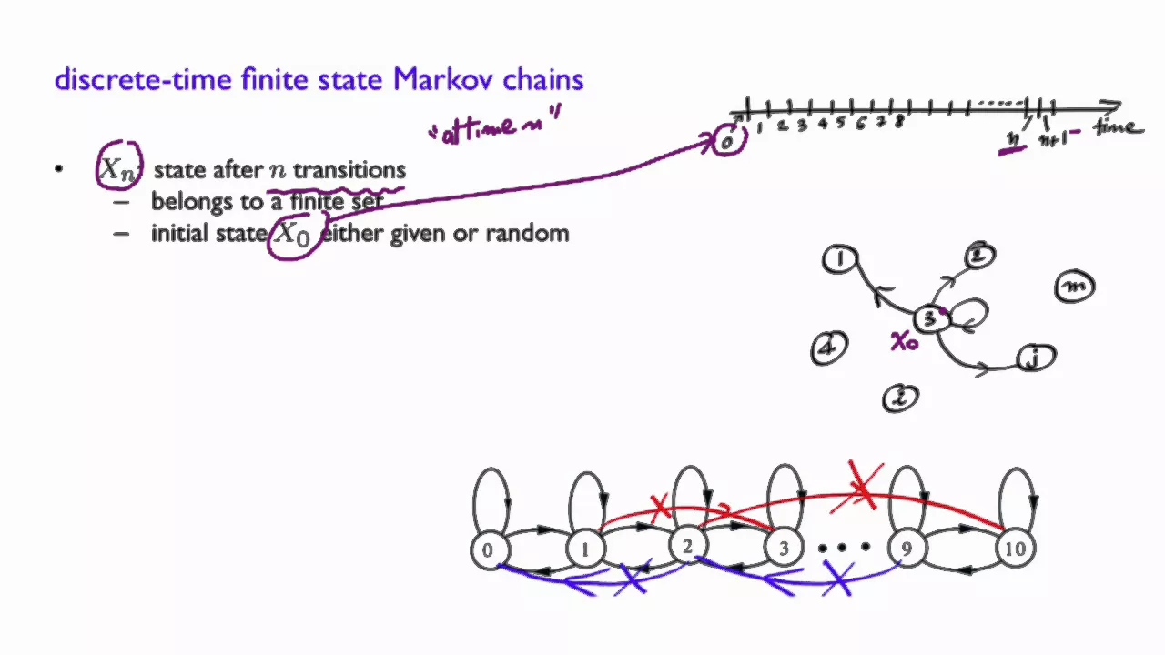


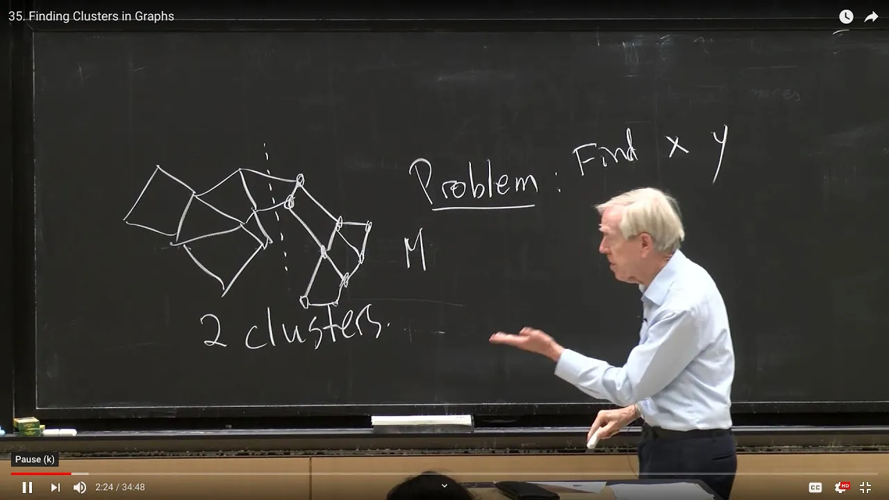


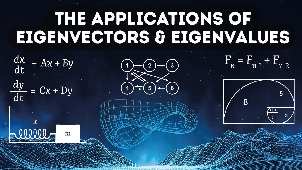






Random walks on undirected graphs converge to a stationary distribution where the probability of being at a node is proportional to its degree, and this process is mathematically equivalent to diffusion governed by the graph Laplacian operator, with the second smallest eigenvalue of the normalized Laplacian determining the rate of convergence and serving as a measure of graph connectivity.
Network Science Lecture 12: Diffusion and Random Walks on Graphs
Added:Linear Algebra foundations, particularly matrix multiplication, eigenvalues, eigenvectors, and symmetric matrices.
Basic Graph Theory concepts, including graph representations via adjacency and degree matrices.
Elementary Probability Theory and the concept of Markov Chains, as random walks are discrete-time Markov processes.
An understanding of physical diffusion or continuous heat equations to contextualize how diffusion operates on discrete graph structures.
Spectral Clustering and community detection algorithms, utilizing the Fiedler vector of the Graph Laplacian.
PageRank and random-walk-based ranking algorithms used in search engines and recommendation systems.
Graph Signal Processing and Spectral Graph Convolutional Networks (GCNs) in Geometric Deep Learning.
Epidemic modeling (such as SIS/SIR models) and opinion dynamics, which model how processes spread over network topologies.
1.9K views40likes1:20:29Original Release: 2020-04-18
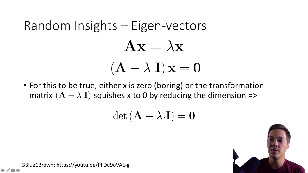
okay so let's get started we're gonna talk a little bit more today about you know about about Russian matrices about you know random walk sort of a little bit more math to kind of give you a little bit more better understanding what those elections are in fact there is like there's there is a lot of work in the last 20 years in math about various usage of krakow questions and in particular you know sort of algebraic graph theory cetera et cetera so we're just going to be just touch the very basics but if you're interested as always there are plenty of literature online on the topic right okay so as I mentioned before we're going to talk about sort of random random walks and graphs and we're going to talk about diffusion and connection in between this Laplace operator the one that the serve laplacian on graph and the actual of las a curator that physicists using and we talked a little bit about also a little bit more about spectral graph theory and normalized laplacian and in fact there were those bounds for lambdas they actually belong to normalize the flash and not just the usual of russia okay so first of all random walk on the graph in fact you know we we talked about this already before when we discussed PageRank because one of the sort of models and approaches to to PageRank is random walk all right and so you should be familiar with this concept but the idea is a random walk on a graph is just a sequence of vertices where each you know where we're starting from we are starting from any node say for example starting from this node um one can go either to this node or this one or this one or this one and that selection is done we formulate random and anytime of the node comes to the second node for example to this one you again repeat this process uniformly at random select where to go might as well go back or go forward and [Music] in this sense this becomes this random wall becomes Markov chain because the next step depends on the current the next position depends on the current position and does not have any memory right any memory of the process so we're also going to look at undirected graph undirected graph so in this case traveling in both direction along the edges are allowed so that that's a difference between this and PageRank computations but that's actually huge difference because when you have undirected graph as you will see the stationary distribution can be easily reached versus when you have a directed graph to reach stationary distribution we actually had to play all kind of tricks I'm getting reads of the things in the graph and also ending this sort of teleportation that would allow you know sir / or the Walker jump from any node to any other node here we don't have that problem okay and so this random walk is defined by probability transition matrix that just tells me the probability of going from one node to another and typically again this probability is just computed by you know having an equal probability to follow on any of the ages that emanates from a node so you know if you think about this random walk you know in onto the surface right onto the plane all that I look typical typically what they're gonna look like you know if we think about a regular graph sort of that's you know the steps of the random walk on a graph now you could try to actually simulate this is trace it on your graph you'll actually see you know similar similar picture so let's do some math here um so we're gonna be considering undirected right connected and for a minute unweighted graphs in general you can actually add weight to the graph sorry guys you sorry things that were supposed to happen at different time always happening of course when you don't need them um okay so back to us to our story so we're considering undirected connected and weighted graph and for this a graph will build this transition matrix is probably the transition matrix and the way we build it is the following if there is an edge in between and AJ between two nodes there is an edge in between them then we set up paj probability of moving from node I to node J um and it is equal to zero if there is no connection so you know if we if I instead of just writing out the nodes and edges if I just use adjacency matrix then PHA is adjacency matrix divided by the node degree and what's important here is to notice that we're going from that we're going from node and the matrix is is when you have a notation a IJ right that notation assumes that we're going from node I to node J right so the walk goes from node I to node J and that's why we normalize it by the degree of the node I right because the whole meaning here is that you're going from the node I in you know possible directions and so you have as many options as degree of that node and so that's why your normalize by the no degree okay and the index I here is because it's going from I to J make sense okay so you can actually write it you know you can write it this way or you can actually put it in you know just as a diagonal matrix and it's just convenient notation he put in t minus one where the matrix is diagonal and that's how we define it then the again very simple math says that the probability that the node that the walk actually sits on the node I at time T right and we can calculate probability of the note of the walk of the Walker of the walk to be at the node J at the time T plus 1 and the way you do it is you just sum up probabilities of being on the neighboring nodes times the transition probability of going from those nodes to transitioning to node J okay so it is a probability of being on node I time the transition to no J and summing from for summing around all the nodes I in the graph okay and so then just plug this in and that's what you get all right and so in matrix form it's a probability of being again them and this is a probability vector because the block can be on any node in the graph right it's just different probabilities from being on different nodes and that's how you compute write probability of being on and on on any node at T plus 1 starts from probably being a node T and that's your matrix now again I want you to pay attention to this we are in fact multiplying of the matrix from the left right I'm the reason for that is because of the indices right if if it says PID ai ai J well this is you take a row vector and multiply by the matrix right so you do it that way that's how it works because this is the first index of the matrix right typically when you do matrix vector multiplication you do it on the second index which means you multiply matrix on the column vector on the right here it's a row vector and we multiplied it on the left okay now of course you can write the transpose of the matrix and multiply you know on the right by the column vector but this is sort of traditional notation in the Markov chains so we keep we keep it we keep it that way now if you think about like modeling and simulation of this for example if you want to think about this as like actual walk right you can say okay I'm starting with P Zero vector at time zero that is you know probability of s terrible of being of being on different notes is zero except for one it is one on one of the notes zero everywhere else and then you're iterating that vector and that changes probability and so slowly your probability from heavy from wizard having a peak of being on one node it kind of spreads around because you know depending on how your telegraph moves right how your graph is arranged before example node has you know four options to go to well it gets 25% from ability to be on each of the nodes and that's vector P is actually that probability does make sense good question yes it is will be not converge in no time I mean that it's seems like a Markov process which cannot be converges some condition yes that's exactly what we're going to be talking about in a minute is if this is gonna converge to a stationary distribution right so if there is when we start with particular distribution right with with maybe in a probability zero on every node and some probability on one node after multiple iterations will we get to the situation when the distribution will start changing right so you kind of apply the separator and nothing changes right now that's means that we get to the stationary distribution and that's what we're gonna do on the next slide okay so let's go to the next slide so as I said we're starting from initial distribution right and then we you know do step by step by step and if we make that T steps the way to you know write it in the way to understand it is that distribution P of T is p0 times the matrix to the power T all right that's T steps now if we have a connected graph and we you know we're not doing any bipartite graphs here then we can show and we're gonna show it in a second that this process this iterations will actually converge to what's called station distribution right and so which means in of its stationary distribution you plug it into this equation and that really means you know this is a definition of stationary distribution which sort of makes sense stationary means you know you apply the same operator I can make another step but the distribution has a change and you know by looking at this you're realizing the business and the fact you know again an eigenvalue problem where is an eigenvector corresponding to them become one sorry guys I have I'll have to take you you know like when when the delivery is it should be in between like 8 a.m. and 24 hours right what's the probability that they're gonna deliver it when you actually doing a lecture for 1 hour during the day well guess what in during this week it 3 times every diamond store the math doesn't work at all I think they just they just know how to do maximum disruption well anyway so we have the the probability distribution and it's stationary right and so in order to find it we really just need to solve Agudelo problem now so far I was just showing you like look this logic of taking the distribution and iterating leads us to eigen the other problem but in fact there is you know there is exists a theorem and we also I think we mentioned it before it's called Courant rubinius theorem sort of it's fundament of therefore the Markov chains and it has like lots of formula lots of different formulations but if you look for like real square matrix formulation and there are several conditions that are satisfied and the conditions are the matrix is stochastic and stochastic and this particular form of a theorem we apply to stochastic matrices but it's actually more in general so if the matrix is stochastic which means the entries are non-negative and rows sum up to 1 and that's what we have because we took our matrix we converted into transition probability matrix by dividing by the node degrees and so that makes all the rows and now matrix to sum up to 1 if it is if the graph is strongly connected and the matrix is irreducible well graph strongly connected to remember it means you can get from any node to any other node and when the graph is undirected right any connected graph is strongly connected and we agreed to look on there on the connected graph so you can get for me so the walk never gets stuck that's what it means and if you well we don't care here because you know when you don't have directions in the graph yeah it is a periodic so all those conditions are satisfied and so the rare exists there exists a stationary distribution which can be found as a left eigenvector and this is again it's a left eigenvector it's a row vector right so it's a row vector a left eigenvector attached I mean you can actually write this isn't right eigenvector but then it has to be that the transition matrix has to be transposed so convector it exists and it's in fact it's unique which is very good so the distribution is unique however you start you always converge to that distribution and in fact the sort of power law iterations which means you know you just multiply by matrix and that's why it works here because of this theorem now the random walk on graphs is actually reversible reversible means you know you can sort of trace it and they can play it back like in the Mooney sort of you know take the frames and play it back and you cannot tell where where you know which was going forward which was going backward right so it's reversible because again because there is no directionality in edges you can reverse any move and practically what it means and that's called detailed balance that is you know probability of being some note and going to its neighbor is equal to probability of being on neighbor and coming back so those two products are equal and that what makes it reversible right oh that's requirement for reversibility so if that is a trick that true and that is a true for our work on a directed graph then just plugging in substituting the definition how we define the the matrix right the transition matrix put it plugging it here you can easily see that this works and remember our graph is undirected so a IJ is a GI so it works only where this ratio is constant and so that means really and by the way you know sum of all the PI's has to be equal to one because the distribution that works only when the P I is equal to the following right you can actually easily calculate this right okay so that means actually very very simple thing if you look at this P I is a probability of being on the note I it is proportional to the node degree and that's pretty much it right so this is very sort of intuitive and naive you know explanation where you actually start walking around and if you can go and be on any node there is a high chance of course to end up on then what you'll spend more time on the node where that has no degree more connections more roads going to it and again remember um this is random walk there is no traps in this walk so it's infinite it's going and going and going and going and so the Walker the walk visits different states but what we observe is a probability right of being particular state probability being in particular state means out of all the states fizz's that you know how was a fraction of visits we're on this particular state on this particular note and so what this says is when you have this random walk on undirected graph the probability of being unknown I is proportional to that note degree right and that's a stationary distribution so the the nodes with the highest degree will have highest probability now this is not true when you have a you know directly graph now when you run page rank on undirected graph this also will not be true because remember was a PageRank we actually had to adjust had to adjust this transition matrix by adding those teleportation jumps right and that makes that that those jumps those teleportation cops they do change the station in distribution all right so PageRank ran on and on on undirected graph will give us different a discrete distribution from this one due to the protected due to teleportation but if we turn that off completely and then yeah then the answer is trivial so the distribution the probability is proportional to no degree any questions here make sense okay okay let me move on now there are different versions of this random walk exists right um and for example there is what's called lazy random walk now lazy random walk means the following the probability of being at a particular getting in a particular node at time T plus 1 is split in between an probability of being on that node and then moving there so which means to be traditionally in the RAM in the random walk for the node being I'm sorry for the world being in a particular node it can only as a next step it can only go to neighbors with this lazy random walk we actually allowing a walk to stay on the node right with some probability in this case it's 50/50 so there is a 50% chance that you're gonna stay on the node and then there is a 50% chance for a walk to go onto the neighboring nodes all right and then you can also show that it always converges and you know just converges to slightly to slightly different angles now what's interesting is that and what sort of interesting in terms of you know mathematics and actually quite practical also interest is to understand how fast how fast your walk converges to the stationary distribution which means if you actually play this sort of you know walking game how long do you need to do this right how many iterations you need to do to see distribution to see this how to get distribution converge to the stationery case right it's kind of it first distribution changes a lot but then change is slowing down and finally you know you get to the stable distribution so the question is how many iterations you need to do before you reach the stability all right and there a theorem for example that deals with this with a second eigenvector you all right okay so so that's the lazy random walk and just so if you look at the distribution and let's say it starts from a particular note right so we actually started from a particular note which means the probability everywhere is zero except for that note and then the probabilities spreads around and increases and goes in across other nodes and so what one can show is that probability of being honor probability of being on a particular of probability of converging or the Dildar the difference in between the probability of being a node and the final distribution actually depends on this nodes degrees and more what's more important it also depends on the second eigenvalue the second-largest eigenvalue to the part taken to the power T what designs is falling over howdy is it no degrees it's no degrees up there are two nodes node I is a node where you started so P sub I the vertex I it's a node or vertex where the random walk started from and J is any other node any other vertex in the graph where you ran where you want to see how fast you know the it will converge right so if you want to see how fast the note I will converge to the final distribution put there the degree of I then that part cancels out it is the best to start with highest Oh degree it best to start up to the cool yes and that sort of if you think about this you want your walk to spread as fast as possible right and that happens if the note has lots of connections right because otherwise it will sort of follow a particular trail here if it's if you start with no the high degree the resolvers you instantly kind of gaining on to the neighboring neighboring nodes okay and so then there's this question about this lambda 2 and so now now I want to remind you that this is a second light that's largest eigenvalues right so compared to the the story with you know the one we did yes last time where we looked at the smallest eigenvalue here it's about the largest eigenvalue all right so lambda 1 is a largest eigenvalue it's equal to 1 lambda 2 is less than 1 because of Toronto ministerium and here we're trying to you know estimate with that lambda 2 right we try and just made the the speed of convergence okay make sense all right okay now now I want to step back okay do you have question guys no all right okay so let's talk a little bit about physics of diffusion so what I want to do now is to connect you know that the physical property is where is the laplacian operator right we kind of talked about it a little bit last time but now I want to make it explicit so just to remind you you know from physics diffusion a movement you know of a substance um you know you can think about the diffusion you know the gas or water or you can even think about diffusion of the heat and typically you know the physics says and it's it's called ficks law that the diffusion happens against the gradient right which means whenever whenever you have material or you know temperature of the higher concentration it's going to diffuse out of there right and so pretty much what this says is that if you have a region of the higher you know high of high concentration of stuff my computer is just not a baby today - well um then the flow will be out of that region out of that area of high concentration so against the gradient and so if you have some you know some stuff and then you have a concentration of that think about you know putting a drop of ink into the water you know there's a high concentration of ink within that droplet and then we go according to the ficks law the flow will be of that ink will be out of that droplet right so that's fixed law then there is a continuity equation which just says that the change in the concentration is connected to the gradient of the flow which means you know you take some stuff out the concentration drops that's you know as easy as that and then when you take those two equations together you take this ficks law and you put it into this continuity equation star box you get a diffusion equation or a heat equation right and that the equation we normally you know see as and you solve quite often if you actually work on some partial differential equations that's sort of classic example and Delta is this laplacian operator right which is double gradient gradient square so that's sort of that's where the physics come from now if we try to model this or apply this physics to to the graph oops so I let let's start to just take this logic and apply it to the situation when you have a graph and when it have nodes and where you have you know if you wish some stuff of quantity per node by the way you know later on we'll see that a lot of predictions that done on graphs they're based on the same idea based on the sort of propagation of something on on graphs right so we can think about the quantity F sub I of T as against some sort of quantity of stuff on the graph on the node of the graph and what we're saying is that that the the amount of this quantity at the time T plus 1 is equal to the amount of that quantity the previous moment of time plus the change and if we're here working with the same ideas as their diffusion right so we're trying to do diffusion then what we're saying is a following this the substance can diffuse can move from one node to another if they're connected so you better connected is this a IJ right so there's a connection between know that I and node J and then the stuff goes from node I to node J from row J I'm sorry to node I and that you know the the amount that flows is proportional to the difference of the values so it's again the same gradient type of the same diffusion type of idea the diffusion happens against the gradient and the rate of the diffusion is proportional to the sort of gradient so the more the higher the difference in between the concentrations right the more will be the flow the faster the wheeler flow the more stuff will flow so the same thing is here we're just saying that the amount of change depends on the difference on those nodes and so if the nodes have the same amount of stuff then there'll be no flow from one node to another if they have different amount of stuff than the flow then there will be flow right and you can actually even without like sort of going through all the math you can imagine that if that's a process was going to be happening after a while so after you run this process for a while on the graph what's gonna what's gonna happen with sort of amount should have equal yeah it should it should yeah exactly it eventually when everything kind of when the process runs for a lot for for a while it will all the nodes which should have equal number of stuff because you know those changes should stop and you know if you think about I don't know heating or again droplet of water you put it into the droplet of link into the water a glass of water you will see how eventually eventually it will spread over the entire glass right or you know you heat a plate of metal and then you know it's gonna be warm all over again so that's pretty much the process but this is sort of mathematics behind it right so you can actually write this now as a differential equation this is your right hand side and you know what's interesting is that the next the next line yes I'm taking the differential equation I'm taking this right hand side I'm just making a very simple change because you know I take the sum and put it into into the formula then I realize that this summation is over J and here we just have a node I right so I can take the sum I can take this node outside of the sound and then summing AAG over J's actually gives me to the node degree the degree of the node I and so that's that's that and then you know I can also take the sum out if instead of just having a degree of the node output there also degree and Delta IJ right so it is the sum becomes di when I is equal to J so these are simple manipulations but what did we get in here right this formula we seen on a previous lecture and that's a graphic question so III g minus dij right we need it last time and so from the sort of very simple physics we realize that if you want to describe the diffusion on the graph your Laplace operator that sort of physics differential of plus operator can be represented as this graph laplacian which is adjacency matrix minus diagonal matrix of no degrees okay and actually that's why it's called laplacian because you know there is this very direct connection with with physics about I see yeah C is some constant the same way as here in the in the ficks law I say okay the flow is proportional to the gradient but we add the constant here and physics is called fix actually constant and that is different for different substances here it's just you know just a constant the number that you come up with and that will actually control in a second you will see that that number controls how fast things you know equalize this is some sense the the you know the speed of the flow right was which things move is it possible that the same no there will be several particles in this mind I know come by the way guys if you have if you have a mic it's better if you ask questions just using the mic is easier so you know how do it how to win understand you know diffusion on on on on the graph right well just you can think about then maybe you know like water pipes right so so the nodes are our you know the bowls where there are waters and there was connected with pipes and then you again drop an ink and it can spread through it alright that might be sort of thing if you know the the visual intuition example be about the diffusion on graph or in other way think about again you know plate and there is you sort of for example by whatever reason it's designed such a way that or you know think about metal frame right and then you're hitting it and then the heat propagates along the wires of the frame and slowly spreads around that sort of the example of also example of the diffusion on graph right it's just wireframe um you know it doesn't necessarily have to be like sort of simple rectangular right it can be anything but practically this is going to be used to actually calculate influence how that propagates on graph or different properties on a graph if you have for examples some properties designed to different nodes and you want to figure out you know that those properties in other nodes that one of the ways you can do it for example I know age of people in social network and I know connect connection and I don't know age for other nodes on the network so the way we're going to predict we talked about predicting of assemblies ages to look at the age of his neighbors or friends but now imagine that you don't know the age of his friends but you know the age of you know friends of friends of friends of friends of friends right in terms of network and so that means you need to take that age information and thread across the network in some consistent manner right that it still satisfies the information on the nodes but also predicts and gives you values for those nodes that are not there or that that the information doesn't is it before in other in other words think about the function that's defined on several separate nodes and then you want to interpolate this function across the entire graph but the way you interpolate is you're interpolating along the ages so that's what this pretty much describes okay all right so that's our graph laplacian the one we talked about before last time and I just bring this up again so we define it as a difference in between diagonal wheels in between diagonal matrix and the Jason C matrix or if we write it explicitly on the dab you know we have no degrees of the diagonals if there are edges there would have minus one and there is zeroes otherwise right so even this is adjacency matrix and then we have degree matrix then here is laplacian matrix okay you know again I coming back to this is because though we first notice we first saw the laplacian matrix in their graph partitioning algorithm in fact you will need it over and over again for example again here in diffusion but in some other algorithms that are related to graph now coming back to spectral properties we also talked about them the spectral properties of a fashion matrix that you know we have the eigenvalues you know we have their non negative and there have orthogonal eigenvectors and the smallest eigenvalue is 0 all right and we discussed it previously and the corresponding eigenvector is a constant all right and the other eigen value eigen vectors will be orthogonal to this one and the eigenvalues will be greater than 0 now couple points here one is the number of zero eigen values is equal to the number of connected components right so if you have one connected component then it's only the smallest eigen vector then it's all on this most I can value that is 0 but if you have multiple connected components then you can just see this by eigen values and the second smallest eigen the second smallest eigen value the one we in fact used previously the one we just discussed last time when we talked about graph partitioning obvious also has a name of algebraic connectivity of the graph it's also called spectral gap it's also called Fidler vector the corresponding reactor cost in director by the name of implementation who actually investigated this in seventies now what's important is is it and that's what we're I gave you the wrong numbers here last time is that if we have a disconnected graph for example that lambda 2 is equal to 0 right as we discussed but if you have totally connected graph it is equal to n and you know I think last time I mentioned I had it equal to 2 right or 1 just a bit strange so it does grow of course with the size of the matrix so that's the main spectral properties now why do we need them well because if you remember when you have you know differential equation like that partial differential equation if you solve it numerically you solve it through find the differences and you know if you do find the differences on the rectangular grid then it is you know the traditional sort of finite differences but if you try to define the differences on a graph where you find the difference in between neighboring nodes then you get your clashing matrix but if you want to solve this equation analytically how would you do that let's say we have this this equation when solved analytically by the way this is of course system of equations right because this goes we have an equation per node right so this describes the first node I'm then their second or third nonet cetera so how would you solve this analytically do remember from math classes a question like situation it amended me ah so you have yeah you want to do it two separate variables but see the challenge here is this is a we have here you know this is not just one equations it's multiple equations right since its locations it snowed fi and this is FJ right and this is a matrix so I mean there is a standard way of doing it right is by trying to express like you said sort separation of variables trying to express solution as a linear combination of basis functions right and so in this case we'll let's take a look at the diffusion equation and again if we were if we were doing sort of physics that would be you know set of partial differential equations where we have derivatives with respect to time and where we have derivatives with respect to X a X Y & Z here instead of those XY and Z derivatives we have the flash and made the Platinum matrix so what we can do is we can actually like you said do separation of variables and right and the solution in the eigenvector basis right in the base I can write eigenvalues eigenvectors we take time we'll put time within the coefficients and these are basis functions right and the basis functions are eigenvalues and eigenvectors of a client matrix then we can easily you know plug it in and do the usual stuff with differential equations right because you do spiration the variables the derivative stays only with those that have time in the you know and then you get equation only for the evolution of the coefficients and then you can get you know write down the solution right as a combination overall basis functions so this is a usual stuff now to the question you had a question previously also you know the role of the see well here it is right so the C will actually control you know the the the pace with which the results will be changing right because we the function of the converging now what's interesting here is that if we look at the solution if we look at the solution we remember and and remember for a second that this is laplace matrix to question so we have all lambdas are greater than zero and the first one is zero right so we talked about it before so which means when time goes to infinity within the some T goes to infinity all lambdas are greater than zero C's are also greater than 0 so this exponents will go to 0 right and there's only one that will survive when time goes to the engine is only one exponent that survives the one that corresponds to lambda 1 equal to zero right that's the only one that survives in here and so the final distribution will look will actually depends on the first eigenvector so the first eigenvector will tells you in the final state you know how much stuff you will have on each node all right now that's like sort of intuitively clear process where you take something and it diffuses now the reason I'm also talking about physical diffusion is to kind of connect this with a little bit with this process that we started the lecture where we talked about you know the walk going from one node to another because if you remember even in physics um there is this sort of macroscopic different description of the diffusion where you talk about you know whether you write differential equations like that but then the results of statistical approaches where you can actually look at the statistics and sort of random Brownian motion and then use that to derive some of the equations so okay here and the picture sort of obvious of this picture you know if if I try to model the diffusion on the graph and this is I'm modeling it on the grid right but any greed is a graph and the idea is that there was a starting you know starting combination where we have in a different sort of level of intensity and then you run this diffusion as a simulation right iteratively it spread spread spread spread spread eventually it's actually will will completely level out you know I didn't wait until the very end here but now we get that in blossom feet here our solution it's not a mirage unit yes exactly and so white everybody let's why is what what is the weight of the friends is so impersonal think you like my advice vector by producers wow you know what's the what the what the goal of doing this right so one you know actually here the goal is to understand the process because of course the most interesting part is if you have different starting conditions how fast you you know you reach certain regimes right I mean the answer the answer what time goes to infinity is clear it's interesting how this process is evolved so that's that the main reason plus I just wanted to show you you know the where and how the laplacian operator actually connects to the physics you know just again kind of why why we want to know for example the process well the reason is you know probably look at that that's the most striking example is like right now with you know infection we do we all know that eventually it should plateau right so the final state is no the final state you know X percent of population isn't as you know is infected right but the question like how that infection actually spreads right and how you will get different parts getting infected you can think about actually diffusion is one of the models you can actually use there right because it propagates along the contacts adjacency matrix so it's for other so here I'm sorry I couldn't I couldn't this is a heat map right so well yeah it is a heat map of adjacency matrix on top of adjacency matrix where adjacency matrix is in this particular case it's just agreed just a regular grid on the regular so it's a regular grid which means every every node has four neighbors etc right so that's sort of easily just done for an example but you can of course do it on you know any graph you want here color stands for different level of intensity x' so you know the red I think those dark brown is just so you can set up remember you know you can set up at different initial conditions and you can say okay you know all the nodes have zeros and then this has initial value or initial concentration you know equal to I don't know 50 this is 20 and resistance so it's just different initial conditions for different parts of the graph and it just shows how its smoothness out that spreads out alright so you know couple sort of observations which you actually already already made but they're this sort of you know instructional right so laplacian operator by itself as an operator it's what's called a you know smoothing operator which means when you apply it to some function it's smooth as it's out now why you know why is that happening and you know we saw it right we'll use you take those initial distribution and then you apply the question apply apply apply and eventually everything flattens out so you just don't want to apply too much but the way it works is is the following if you again I'll just take this laplacian operator right and I apply you know I put it in - you know explicitly the difference is between diagonal and the adjacency matrix I again just write it out and then I you know pull out the node degree and so what it says really it says the following when I apply a laplacian operator to a node what happens it takes the value of the function on that node and subtracts the average of the function on the neighbors right so even if there is a node and then there is neighbors right what it does is literally takes the value on the node and subtract the average on the neighbors that's moving the value on the note to towards the value of towards the average of the neighbors so that's what it does you can also understand it from this your matrix which is you know what we use also by the way on when we looked for a graph partitioning right but if you look at this bipartite I'm sorry if you look at this form right where it is again you take this motion operator and make a quadratic form out of it you realize that this quadratic form is going to be minimized for example when the neighboring nodes will have similar values right and this quadratic form directly relates to the eigen in vectors and serve the smallest eigenvalue will correspond obviously to you know although all the notes getting the same value which is if you remember against most I can tell you the smallest eigen vector in that case was all wats right and the second smallest and gives us also very smooth solution so you know there is sort of no magic in this it's just all those things are connected right and when people do regression on graphs they very often use this type of approach right and this is sort of you know though though we started from this sort of physics and math but again if I ask you sort of naively intuitively let's say I want you want to predict somebody's age um by knowing his contacts you know what would you do you probably take it Scott you know how would you predict this somebody's age you take his contacts right and you probably kalki calculate the average age of of his friends and that's gonna be your predictor but that's literally what this does right it to calculate it it pushes the value and and of the node to the value that is average of the neighbors and then if you'd apply this repeated iteratively and repeatedly to all the nodes it eventually of course levels them up make them all have the same value okay all right so couple more things is this normalized laplacian you know those of you who might get sort of interested looking in-depth into this topic might might meet a lot of this sort of normalize the flesh and stop now and in fact normalized laplacian is what allows us to connect those random walks and this physics of diffusion so the way normalized laplacian are defined he is through well normalization of laplace matrix right so you take the this L matrix and then you scale it the following way now it's kind of interesting way to do it the reason you do it this way instead of just multiplying by for example D minus one is because you want normalized laplacian to also remain symmetric so if you do that here is your definition it has ones on the diagonal it has this value which is minus one divided by the node degrees when there is an adjacency and has zero otherwise right um just so you just to remind you I'll go back for a second you know the the definition of graph laplacian is diagonal degree on the diagonal minus one of the diagonal and zero where there is no connections and so here we make a in such a way that diagonals are equal to one so that's called normalized laplacian and then with very simple mathematics you can actually show that the random walk matrix right the one that we started with traditionally that is d minus 1 times a you can actually show that is equal to this expression where this L is normalized laplacian now why is this important well because if you learn the ramp a little bit of thing in algebra what you do is you take when they take a matrix and multiply by inverse on one side and other matrix on the other side right that actually is called similarity similar to its similarity transformation right and those similar matrices have a lot of similar properties and for example you know that relates to his eigenvalues and so there is it's not a you know an accident that when we started with transition when we looked at the transition probability transition matrix the random walk matrix will look at the maximum eigen value and is equal to 1 it's actually corresponds to smallest eigen value equal to 0 in normalized laplacian okay i don't want to go a lot into the details here you know if you're interested I'm Ian um just wanted also to point out that there was some you know interesting properties that one can have for this normalized laplacian so first of all for normalized laplacian and by the way this was that what i mistakenly put last time on the slides so for normalized laplacian um all eigen values they are in between zero and two right and here it makes sense because there since it's a normalized matrix and the scale is already removed but what's more interesting is this what's called Chickering equality and the conductance now conductance we actually looked at that property that property remember when we when we talked about the graph let's say there is a you know well yeah it's hard to draw sorry guys well there was a graph and then you partition this graph with the graph cut you can calculate just either the number of edges that crosses that cut right that room that you need to remove to split the graph into two pieces or we talked about normalized cuts where you take this number of edges and then you divide by the for example you know degree of the nodes or um there was also what's called conductance where you take the sky and you normalized by minimum of two of what's called volume of the cut and volume is the sum of the node degrees in the set or sum of all the edges so so one can show that this the minimum value of that cut is actually bounded by this second eigen value of normalized laplacian now why is this important well because [Music] this conductance right or this cut tells us how good offer separation of a graph you can have right so it pretty much tells you if the graph have some good clusters that you can find by splitting the graph and conductance is a measure of it right if you have very good clusters those cuts will be small so what this formula says is that the smallest no this is a smallest possible cut it's bounded and it's bounded by this eigenvalues so what it says literally even the second eigenvalue is small there might be good clusters within the graph and you know you should be able to find that but even this lambda 2 is large then your graph does not have good clusters in it and there is no good way to partition it whatever out with me Ron you will never get good fasters so that's actually a very strong statement and very useful so you can actually take the matrix take the graph you know you laplacian matrix you'll normalize the prussian calculate this lambda 2 and depending on the size of the lambda 2 you can it tells you the bound um it tells you whether you're gonna have a good partition or not alright okay so uh and again thanks for bringing up last time you know the you know the wrong numbers here so I could actually would look up and correct things I think that's pretty much all so today it was again you know another sort of mathematical part of the lecture but there is a like really really deep literature on graph partitioning on the spectral graph theory algebraic graph theory and if you're interested in the connection between this random walks graph you know but just like literally almost almost there you know subfield of mathematics that is devoted to it so if you're interested you know that mean this is a sort of that some some references that can help you get started and the next lecture we will go back to you know overview of clustering algorithms and some other things that you do on graphs any questions you know I would like to know if we will have to calculate eigenvectors eigenvalues class on any exam because it's really been naturally like 10 or more years since I've done native algebra or is it enough to know oh you're just going to look for in a second it's a bit of a question and I was like homework if we need to do okay look I'm not done I'm sure I'm sure on the computer you can calculate that can do second excess of matrix right that's not a problem now the question is if you can calculate the eigenvalues eigenvectors by hand right I I don't remember if we if we kept that in in the exam or not but if we did maximum what you need is to to remember how to calculate it by the matrix for matrix 3x3 and I think you should be able to do it for 3x3 right remember I should so I should remember yeah come exam time there's the time and everything so come on like some homework or I will look for some homework myself but we'd like to know thankfully I ever spared this on the midterm this is yeah this is again if the matrix 3x3 and you write down the characterisation equation and they usually in those questions they usually design in such a way that it becomes a quadratic equation because one usually one eigenvalue is easily found and then i you know i hope you guys still remember how to solve quadratic equation right ax squared plus BX one was looking this up the other day so I can say for sure so yeah I don't - good okay so you do know and then whether you have when you found them when you found I can values you can plug it back into the matrix and find eigen vectors so but again I don't admit them you know I'll check but I doubt even if we had it it was ever more than three by three matrix so you know you're saved there all right anything else so I have a question about what does the math intuition behind it this is that we just second eigen react or not sure not face maybe Chilean equation well you know there is some some intuition right to this and the intuition is imagine imagine that you have a string a string let me try to draw this let's say there is no it's not working today for me so let's say you have a string fix in between two walls right and you know like a guitar string and then you pluck it and let it go and it start oscillating and remember for the string you will get actually if you remember a bit from physics you will get what's so called harmonics right you will get it's symmetric but it doesn't work you have you know first harmonic which is this way right and then you have a second harmonic right and then you can have a third harmonic and so on so the the intuition is that it's actually second eigenvector that describes second harmonic and the second harmonic in some sense pleats your string into two parts right it's a part where we goes up and then the wave goes down and so that's why it is you know that's why it's second harmonic and by the way the way I drew it though you know it's accidental but if your string has non-uniform mass then it's not necessarily split in the middle by this second harmonic but the split will be shifted depending on the distribution of the mass so the idea of the second I can I mean intuition behind second eigenvector is that that the first one just give you the first harmonic second gives you a second harmonic which has a node in the center in the century if it's uniform and not in the center if it's not uniform and that's why you can actually use it to speed this string into two pieces let's make some sense a little bit so so it's like physical intuition about it yeah yeah it's it's it's physical intuition behind it and again like thinking about strings okay I said string but you can think about string as a bunch of masses you know like masses connected with Springs also you know if you remember from physics some sort of you know the favorite usually in mechanics you know you try to solve those type of systems where you have bunch of Springs connected a mass is connected with Springs and you can also think about the system how it oscillates and how you can you know how this eigenvalue helps you to you know find the parts that goes say versus goes down that's that's the main idea right so that's one second I can value doing it consider the third eigen value if we want to split in three clusters and people have tried to do it and sometimes you see that sometimes you know it doesn't work too well yeah there are people people trying to use there are several ways people trying to use you know the separation one is as we discussed previously stake the second eigenvalue I'm sorry taking the second eigenvector and just split it by you know above zero below zero and then you can also within the second eigenvector try to see maybe there is some sort of gaps in the values right and then you group by those gaps and then split by those gaps the other way is to take maybe second and third eigen value and look at two-dimensional space and see if there's any groupings there another way just take the throat again value and see where those gaps are in third and valiant speed buy them again this is this is more of you know more of intuition right but you yes you will see people using a higher sort of the fundamental mathematics the way we described it is about this second eigenvalue right and by the way this is done by by fiddler in this 1973 paper and the rest all this higher levels maybe there are some you know some fundamental stuff unknown about it but you will see a lot of people are kind of experimenting with it I don't think I mean I don't know one another where of very solid sort of you know proves there except for I'm Sophie except for this intuition so it's just a miracle in the division it's not must um the groove to it again and I haven't seen maybe there is some proof somewhere right I've seen people using you know third and then you know and again we're using like the you're actually projecting this in a in low dimensional space in fact laplacian operator is also used a lot to project you know nodes in low dimensional space the reason is again if you look if you look back here what it will force you to do is for no for for you know if you think about in this case if you think about FIS and fj's as B coordinates for example it actually forces coordinates of the nodes that are connected it forces them to be next to each other you these are coordinates right so there is principal component Alice's that allows you to embed something in you know dimensions which is assigned embedding means you take a graph and you want to assign to the graph nodes you want to assign coordinates right because you want to draw a graph on you know on paper and one of the ways to assign those coordinates is actually compute eigenvalues eigenvectors of laplacian matrix not adjacency matrix and then take this for example first laplacian vector its x second reflection vector as y-coordinates and then you draw your graph you control the nodes based on those values and you know looking at this that the iterations right now you realize that laplacian will force those nodes that are connected those nodes that are connected for this thing to be the small at minimum and that's what you you know you remember finding an eagle eigenvalue second lectures comes from optimization problem right so we're trying to minimize this for this to be minimal what's needed is for neighbors and a IJ it means you know there is a neighbor they should have those values close to each other and so what happens it project them on the plane close to each other so that connector becomes close to each other now um it actually it works um but you know for some graphs it works for others it does not because it though it for close notes to be next to each other it does not force those notes that are not connected to be far away from each other and so it's you know it's better it I mean it's it's embedding you can try it sometimes it for some type of graphs it works for others it will not but if you look for the google laplacian embedding for example that term really means calculating eigen values eigen vectors of laplacian matrix and assigning to the points or to the notes the coordinates which are second eigenvector second maybe second third eigen vector from the laplacian all right okay all right guys even there's no more questions we're done for today somebody was asking me about recording you know it's gonna be out there yep
Up Next

23:49
Algebraic Connectivity and Fiedler Vector Explained
@nptel-nociitm9240
163 views•2025-11-13

4:43
Elliptic Curve Cryptography Explained: ECC, ECDSA, ECDH
@PracticalNetworking
28.5K views•2024-10-21

10:44
Fourier Series Introduction: The Big Idea Explained
@DrTrefor
387K views•2021-05-03

6:00
The Mathematical Impossibility of Accurate World Maps
@Vox
23.3M views•2016-12-02
Related Study Plans & Knowledge Roadmaps
Structured learning paths in Mathematics
mathematics
Tensor Calculus: Vectors to Riemann Curvature
01Mathematical Foundations: Linear Algebra & Calculus
02Covectors, Dual Spaces, and Tensor Basics
03The Metric Tensor and Index Gymnastics
+ 2 more learning modules
40h5 modules
Explore Roadmap
mathematics
Gödel's Incompleteness: Logic, Proofs & Limits
01Introduction to Formal Systems & Hilbert's Dream
02Set Theory, Cardinality, and Cantor's Diagonal Argument
03Arithmetization and Gödel Numbering
+ 2 more learning modules
14h5 modules
Explore Roadmap
mathematics
Galois Theory: Fields, Groups & Solvability
01Foundations of Abstract Algebra: Groups & Fields
02Polynomials & Field Extensions
03Splitting Fields & Symmetries
+ 2 more learning modules
24h5 modules
Explore Roadmap
mathematics
Non-Euclidean Geometry: Models & Geodesics
01Euclid's Fifth Postulate and the Birth of New Geometries
02Hyperbolic Space and the Poincaré Disk Model
03Geodesics: Defining Straight Lines in Curved Spaces
+ 2 more learning modules
15h5 modules
Explore Roadmap