A Warren truss bridge made from balsa wood with approximately 30cm span successfully supported over 10kg of load during a classroom load test, demonstrating the structural efficiency of the Warren truss configuration in distributing weight across interconnected triangular elements.
Warren Truss Bridge Load Test | Balsa Wood Engineering Project
Added:Deep Dive
Basic principles of static equilibrium, including how forces and moments balance in stationary structures.

Kräfte- und Momentengleichgewicht - Fachwerke und statisches Gleichgewicht 7
155.3K
A system achieves equilibrium when forces and moments are balanced, preventing motion or rotation. For planar systems, three independent equilibrium conditions must be satisfied: ΣFx = 0, ΣFy = 0, and ΣM = 0. The force equilibrium requires that the vector sum of all forces equals zero, with separate conditions for each perpendicular direction. The moment equilibrium requires that the algebraic sum of all moments about any point equals zero. Support forces are conventionally drawn as positive values, while weight forces are negative. The reference point for moment calculations can be chosen strategically to simplify computations, typically at support locations to eliminate unknown reaction forces from the moment equation.
Click to watch →

Homework | STATIC | follow parallel forces | 3rd sec
274
Static equilibrium requires two conditions: (1) resultant force equals zero (ΣF = 0), meaning upward forces equal downward forces; (2) resultant moment about any point equals zero (ΣM = 0). For a system in equilibrium, forces balance in opposite directions, and moments balance about any pivot point. The moment equation includes all forces multiplied by their perpendicular distances from the pivot, with appropriate sign conventions (clockwise negative, counterclockwise positive). These principles apply to all static equilibrium problems, from simple beams to complex structures.
Click to watch →

CCEA GCSE Further Mathematics Mechanics Specimen
1.5K
This section covers static equilibrium principles: (1) For an object in equilibrium, the sum of upward forces equals the sum of downward forces; (2) For a uniform plank with masses 5 kg, 3 kg, and 4 kg, total downward force is 12g = 120 N; (3) The sum of clockwise moments equals the sum of anti-clockwise moments about any pivot point; (4) Taking moments about pivot C: clockwise moments = (1.5 × 3g) + (5 × 4g) + (2 × 5g) = 345; (5) Anti-clockwise moment = 3.5 × R2, giving R2 ≈ 41.43 N; (6) Reaction at C is R1 = 120 - 41.43 = 78.57 N. These principles allow calculation of support reactions in static structures.
Click to watch →

일반기계기사 1차 필기반 인강 강좌
1.6K
This section covers the principles of static equilibrium essential for analyzing stationary structures. The instructor explains that for a body to remain stationary, two conditions must be satisfied: (1) The sum of all forces in any direction must equal zero (ΣFx = 0, ΣFy = 0), ensuring translational equilibrium, and (2) The sum of all moments about any point must equal zero (ΣM = 0), ensuring rotational equilibrium. The concept of moment (torque) is introduced as the rotational effect of a force applied at a distance from a pivot point, calculated as M = F × d. The instructor demonstrates how to apply these principles to solve practical problems involving forces and moments, emphasizing that mastering these fundamental techniques is essential before proceeding to more advanced topics.
Click to watch →

Static Equilibrium
273
Static equilibrium is derived from Newton's second law, where the sum of forces equals mass times acceleration. For static structures, this sum equals zero, representing balance of forces and conservation of linear momentum. For any body in 2D or 3D space, both balance of forces and balance of moments are necessary. Forces create translational tendency regardless of placement, but only forces not passing through the center of mass create rotational tendency.
Click to watch →
Deep Dive
The conceptual difference between tension (pulling forces) and compression (pushing forces) in structural members.

Dr. Britt explains engineering straw towers
43.3K
Tension is the force that stretches a member, attempting to pull it apart. Compression is the force that squishes or pushes a member's ends closer together. These are two fundamental ways to load structural members.
Click to watch →
CLASE 4 - SOLDDURA 3D
508
Structural members can experience tension (pulling forces) or compression (pushing forces) depending on how they are loaded. The instructor explains that when a member is being pulled, it experiences tension, while when it is being pushed, it experiences compression.
Click to watch →

2026 Combined Maths Revision by Dr. Pantaleon Perera
955
When a structural member is pulled from both ends, it experiences tension (ආතතිය). When pushed from both ends, it experiences compression (තෙරපුම). These are the two types of internal forces that members can experience. Understanding whether a member is in tension or compression is crucial for determining its structural behavior and ensuring it can safely carry the applied loads.
Click to watch →
Equilibrio de Fuerzas - Física, Tippens 4.40
14.9K
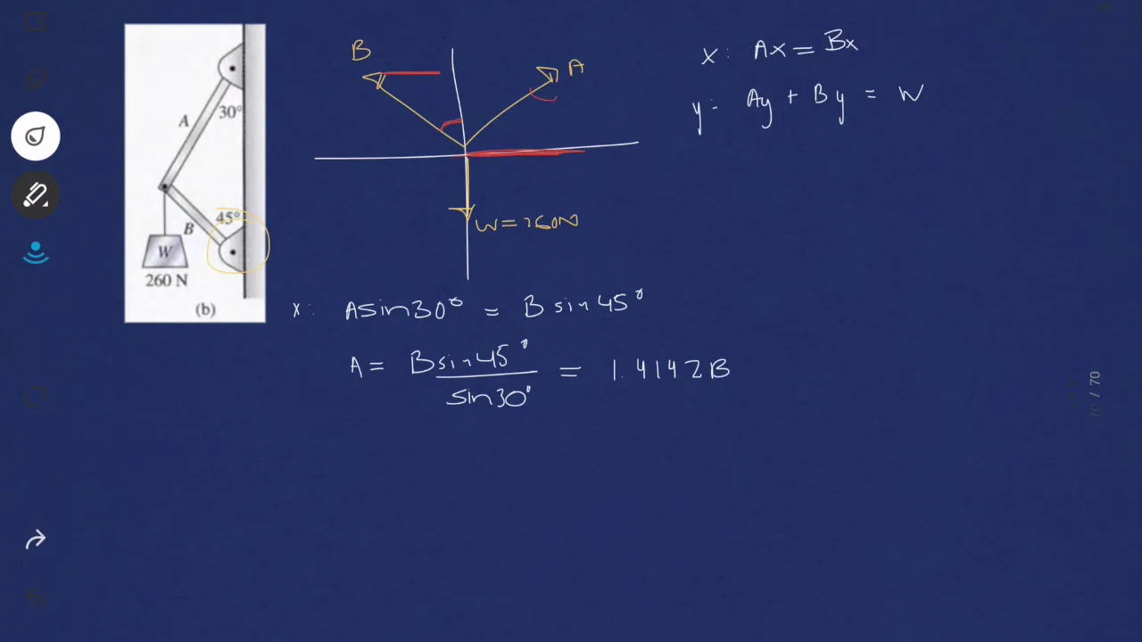
A structural member experiences tension when it is being pulled apart by forces acting in opposite directions along its length. Conversely, a member experiences compression when it is being pushed together by forces acting toward each other along its length. In this problem, cable A experiences tension because it is being pulled by the weight, while cable B experiences compression due to the combined effect of tension from cable A and the weight.
Click to watch →

Estática (Treliças) - Determine a força em cada membro da treliça mostrada na Figura 6.8a
110
In structural mechanics, tension and compression are distinguished by the direction of forces acting on a member. When a force acts downward on a member and the reaction force acts upward, the member is being compressed. Conversely, when a force acts upward on a member and the reaction force acts downward to maintain equilibrium, the member is being pulled or stretched, which is called tension. This fundamental distinction is essential for analyzing truss structures and determining how members will behave under load.
Click to watch →
Deep Dive
The unique material properties of balsa wood, including its high strength-to-weight ratio and directional grain sensitivity.

How Balsa Wood Became the New Gold Rush: From Seeds to a Billion-Dollar Industry!
439.3K
Balsa wood can be divided into three types based on grain patterns: A grain, B grain, and C grain. Interestingly, grain direction controls the rigidity or flexibility of a Balsa sheet more than its density does. B grain is considered best for wind farms and many products because it possesses qualities of both A grain and C grain.
Click to watch →

Balsa wood | Balsa wood Types | Balsa wood Used? |Balsa wood properties | Balsa Sheets Production
7.7K
Balsa wood is one of the lightest woods available with a very high strength-to-weight ratio, making it ideal for aeromodelling and aircraft construction where structural designs can reduce weight by 30%. The wood is available in sheets (10cm x 100cm) with thickness ranging from 1mm to 10mm, as well as blocks for craft and architectural purposes. Different types of balsa wood are available for various aircraft regions based on their physical properties, with some types being common to multiple regions. The wood is flexible and suitable for motion jobs, and manufacturers produce specialized components like spars, trailing edges, and leading edges. When purchasing, it is recommended to order one extra sheet to account for potential shortages during construction.
Click to watch →

Sustainable Composite Materials: Flax Canoe Bio Resin Infusion
166.6K
End grain Balsa is manufactured with the wood grain running vertically from top to bottom surface, maximizing compressive strength which matches how a core is loaded in a sandwich structure. It consists of blocks supported on scrim, allowing it to follow tight curvatures and providing a path for resin flow during infusion. Despite being a natural and sustainable material, end grain Balsa has one of the highest strength-to-weight ratios available in composite core materials and cuts and shapes easily.
Click to watch →

The BEST Fiberglass Deck Core Materials (And How To Choose)
61.3K
Balsa wood offers nearly twice the shear strength of plywood due to its vertical cell orientation, which provides superior bonding with resin and prevents slip planes. Its density ranges from 6-9 lb per cubic foot, resulting in an excellent shear-to-weight ratio. However, water absorption is a significant concern as saturated balsa can hold 600% water by weight and will rot over time. Insulation is moderate at R2 per inch. Balsa works well with standard tools but requires pre-saturation with resin before installation to prevent dry joints. Cost is approximately $7.50 per square foot, and it is available through fiberglass suppliers and boat building specialists.
Click to watch →

El imperio Eólico Chino de 60 mil MILLONES tiene un GRAN PROBLEMA
36.9K
Balsa wood, native to South American rainforests with Ecuador holding 80% of international market share, possesses unique properties making it ideal for industrial applications. Growing to 20-25 meters with trunks up to 90 cm diameter, it has a density of 150 kg/m³—lighter than cork yet maintaining resistance. With compression resistance of 112 kg/cm², static bending resistance of 245 kg/cm², and elastic resistance of 11,600 kg/cm², it enables manufacturing of wind turbine blades, automotive components, musical instruments, and aircraft. Wind turbine blades require increasing length without weight increase, achieved by combining balsa with fiberglass and carbon fiber composites. A 100-meter blade requires 1,200-29 kg of balsa wood.
Click to watch →
Deep Dive
The geometric stability of triangles as the fundamental unit of truss design compared to other polygonal shapes.
Baumechanik I / Technische Mechanik I, Video 22: Fachwerke, Knotenpunktverfahren
9K
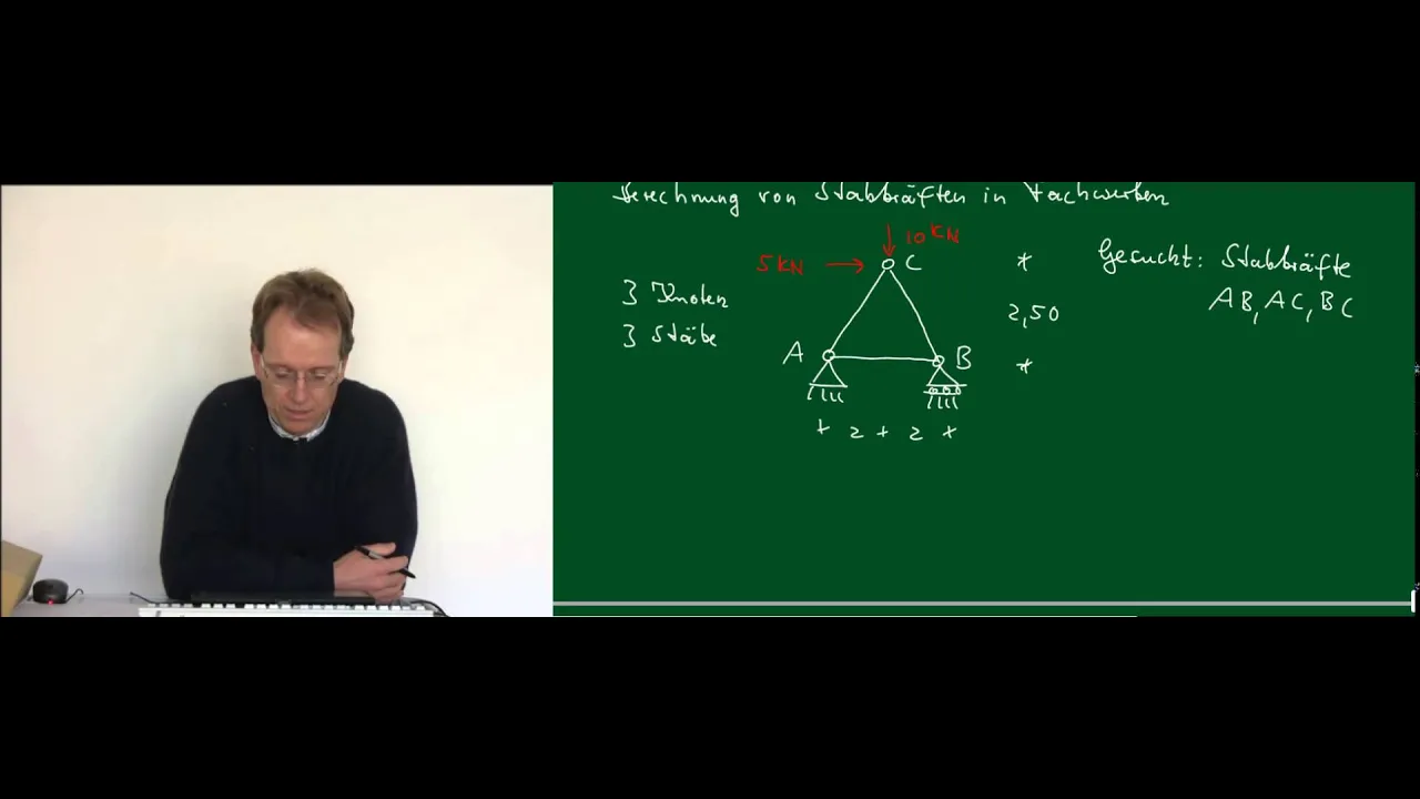
Trusses are composed of triangles because the triangle is the simplest geometric form that is internally stable. When fixed at three points, a triangle becomes statically determinate and can be loaded without deforming. In 3D space, the tetrahedron (four nodes, three faces) is the simplest stable spatial form. Quadrilaterals are not internally stable even when fixed at three points because they can deform into a parallelogram-like shape (Gelenkkette). Due to the pin-joint assumption, forces in truss members must act along the member axis; any perpendicular component would cause rotation. Therefore, each member experiences only axial forces (tension or compression).
Click to watch →

Introduction to Trusses L - 18 | Engineering Mechanics | GATE 2022 | K2K Batch
53K
The triangle is the fundamental shape of trusses because it is rigid and non-collapsible. A single member connected by a pin joint will collapse under load, but when two members form a triangle, they become rigid with no relative motion between members. All practical trusses are constructed by connecting multiple triangles together to create stable structures.
Click to watch →

Why Basic Shape of Truss is TRIANGULAR ?
2.1K
Truss structures use triangular shapes as their smallest unit because triangles are inherently rigid and stable, whereas rectangular shapes are unstable and can collapse under load. With three fixed-length members, only one triangle can be formed, ensuring structural integrity. In contrast, four fixed-length members can form infinite rectangles, making them non-rigid and unsuitable for load-bearing applications.
Click to watch →

Steel Structure roof truss | Steel Frame construction | 3D animation
126K
The triangular shape is fundamental to truss design because it is the only polygon that cannot be deformed without changing the length of its sides. When multiple triangles are connected in a truss system, this geometric property ensures that the entire structure remains rigid and stable under applied loads, making it ideal for spanning large open spaces.
Click to watch →
TRUSSES: Method of Sections (MOS) | Statically Determinate vs Indeterminate vs Unstable | Triangles
16.2K
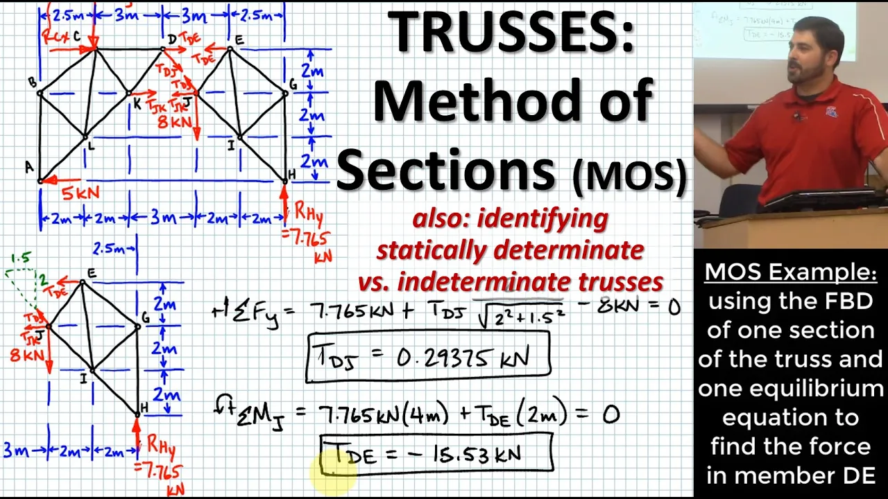
Triangles are inherently stable structural shapes because when you specify the length of all three sides, the resulting triangle is unique and cannot change its shape without changing the length of its sides. In contrast, four members arranged with pins at their ends can form infinitely many different shapes while keeping the same side lengths. This geometric property makes triangular arrangements ideal for creating strong, rigid structures that resist deformation under load.
Click to watch →
Prerequisite Knowledge
- Concept 01Basic principles of static equilibrium, including how forces and moments balance in stationary structures.
- Concept 02The conceptual difference between tension (pulling forces) and compression (pushing forces) in structural members.
- Concept 03The unique material properties of balsa wood, including its high strength-to-weight ratio and directional grain sensitivity.
- Concept 04The geometric stability of triangles as the fundamental unit of truss design compared to other polygonal shapes.
Subsequent Learning
- Step 01Analysis of structural failure modes, such as member buckling, joint shearing, and adhesive de-bonding.
- Step 02Comparative study of alternative truss configurations, such as the Pratt, Howe, and K-truss designs, to evaluate efficiency.
- Step 03Introduction to Finite Element Analysis (FEA) software to digitally simulate load distribution and predict failure points.
- Step 04Real-world structural engineering considerations, including dynamic loads (wind, traffic) and scaling up from model materials to steel and concrete.
Initial Warning
Price Check
Testing Limits
Capacity One
Counting Progress
Stability Goal
Growing Capacity
Locating Focus
Approaching Peak
Final Count
Initial Warning
0:09Playing Section
- 1
A caution is expressed about a potential harmful action.
- 2
The warning is delivered briefly, without elaboration.
The Limitations of Scale-Model Balsa Testing in Structural Engineering
While balsa wood truss projects are excellent educational tools, they present a misleading representation of real-world structural engineering due to the 'scale effect' and material anisotropy. Balsa wood possesses an exceptionally high strength-to-weight ratio that does not scale linearly to materials like steel or reinforced concrete. Furthermore, in micro-scale testing, the structural behavior is dominated by static live loads, whereas real-world bridges must primarily support their own massive 'dead load' and dynamic forces like wind and traffic. Consequently, failure modes observed in balsa models—such as simple joint shear—rarely align with the complex buckling, fatigue, and environmental degradation challenges faced by full-scale infrastructure, limiting the project's real-world predictive value.
Deep Dive
Analysis of structural failure modes, such as member buckling, joint shearing, and adhesive de-bonding.

Building Prototypes part 13 of 18 Large Structures
61.3K
Proper adhesive joint design must avoid peel mode at all costs. Three failure modes exist: shear (load parallel to joint, strongest), tension (pull perpendicular, weaker), and peel (load along line, instant failure). Peel concentrates stress on zero-area lines causing immediate breakage. Shear distributes load across entire area. A properly designed shear joint at 1/10 scale failed at 2 tons; full scale would handle ~200 tons. This demonstrates that properly designed adhesive joints can provide substantial structural capacity while remaining lightweight and reversible.
Click to watch →
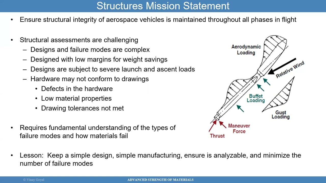
14 Advanced Strength of Materials - Failure Modes
775
Bonded joints fail through cohesive fracture (within adhesive), interfacial failure (adherend-adhesive interface from poor prep), net section, shear out, bearing, cleavage, tearing, and pull-through. Best practice designs joints to fail adhesively before metal substrate. Composite sandwich structures fail through core failure, face sheet delamination, fiber breakage, and ply separation. Bolted connections experience bearing damage and bypass loading analyzed via strength curves. AA 587 investigation found vertical stabilizer failure from loads beyond ultimate design limits.
Click to watch →

Oct 2021 –Timber connections – the European Yield Model explained – Pierre Quenneville
3K
Single shear joints have one shear plane, while multiple shear planes require treating them as multiple double shear units. For single shear, six failure modes exist: (A) embedment failure only in bottom member; (B) embedment failure only in top member; (C) embedment failure in both members with rigid fastener; (D) plastic hinge near top member; (E) plastic hinge near bottom member (mirror of D); (F) two plastic hinges with combined embedment failure. Equations involve embedment resistances (f1, f2), member thicknesses (t1, t2), fastener diameter (d), beta ratio (f2/f1), and fastener yield moment (My). Calculations require spreadsheets or MATLAB due to complexity.
Click to watch →

Adhesive
193
Adhesion occurs through mechanical interlocking (adhesive penetrating substrate pores) or chemical mechanisms including covalent bonding, electrostatic forces, van der Waals forces, and moisture diffusion. Failure modes include cohesive fracture (crack propagates within adhesive), adhesive fracture (debonding at interface), mixed fracture (combination of both), and substrate fracture (adhesive tougher than substrate). Understanding these mechanisms guides material selection and joint design for reliable performance under various loading conditions.
Click to watch →

Four Modes of Failure of a Shear Joint - Aircraft Structural Analysis Video 2.0
650
Aircraft shear joints can fail through four distinct modes: (1) shear through the fastener cross-section (P = πr² × allowable), (2) bearing failure at the hole wall (P = diameter × thickness × allowable), (3) tear-out failure at the edge margin (P = 2 × (edge margin - s) × thickness × allowable), and (4) additional shear planes in multi-fastener configurations; while schools typically teach only the first three, real-world applications require understanding all four modes for proper structural analysis.
Click to watch →
Deep Dive
Comparative study of alternative truss configurations, such as the Pratt, Howe, and K-truss designs, to evaluate efficiency.

Howe vs Pratt Truss Design: Structural Engineering Lecture
126.4K
In bridge truss design, the Pratt truss (with diagonals under tension) is more efficient than the Howe truss (with diagonals under compression) because tension members can be made thinner without buckling concerns, while compression members require additional reinforcement to prevent buckling; this topology optimization allows for approximately 33% weight reduction in the Pratt configuration compared to the Howe configuration.
Click to watch →

Understanding and Analysing Trusses
3.6M
Three classic bridge truss designs emerged in the 1840s: (1) Howe truss—vertical members in tension, diagonal members in compression; less cost-effective because thick diagonal members are long; (2) Pratt truss—vertical members mostly in compression, inner diagonals in tension; more cost-effective since longer tension members can be thinner; (3) Warren truss—based on equilateral triangles, all members same length for construction efficiency, uses fewer members overall, but has long compression members requiring careful design.
Click to watch →
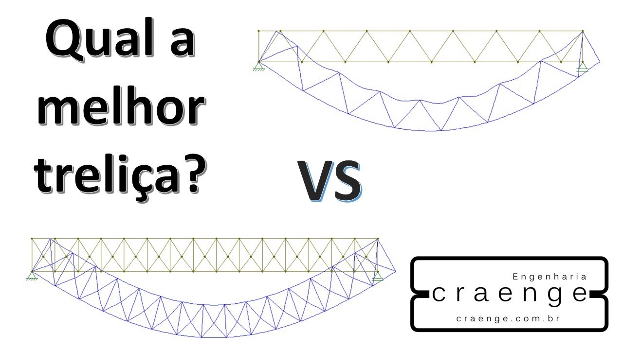
Qual é o Melhor Tipo de Treliça?
7.5K
Common truss types include: (1) Pratt truss with diagonals in the same direction and vertical members, (2) Howe truss with diagonals in opposite directions and vertical members, (3) Warren truss with alternating diagonals without vertical members. Truss height is pre-dimensioned using empirical formulas: height = span / 15 to span / 8. For a 10.5m span, this gives 700mm to 1312mm height. The span/15 ratio is commonly used for economical designs. Truss weight comparison shows: (1) Pratt, Howe, and Warren trusses have similar weights, (2) Warren truss is 24% lighter than Pratt and Howe trusses, (3) X-truss without proper node connections performs similarly to other configurations. The Warren truss offers the best weight efficiency among traditional configurations.
Click to watch →
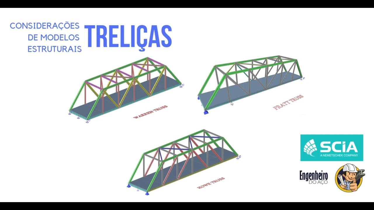
QUAL O MAIS ECONÔMICO TIPO DE TRELIÇA PARA PONTES E PASSARELAS?
9.3K
The Pratt truss is the most economical bridge truss system because its diagonals are inclined toward the center and are in tension under normal loading, whereas the Howe truss has diagonals inclined upward from the supports that are in compression (making them more susceptible to instability), and the Warren truss alternates between compression and tension diagonals, resulting in higher material costs; analysis shows Pratt trusses weigh approximately 10 tons while Howe trusses weigh about 11 tons (13.4% increase) and Warren trusses about 12 tons (20% increase), demonstrating the Pratt truss's economic advantage due to its tension diagonals.
Click to watch →

Treliças Pratt e Howe em galpões estragam o projeto - Enquete 32% acerto - Eng. Estrutural
1.7K
Efficient truss design requires diagonals to have an inclination angle between 30-60 degrees (ideally around 50 degrees) to minimize both structural forces and material costs; the Warren truss configuration with diagonals at approximately 54-61 degrees is superior to Pratt or Howe trusses for roof structures because it reduces diagonal length, decreases member forces, minimizes deformation, and allows for lighter structural members while maintaining structural integrity.
Click to watch →
Deep Dive
Introduction to Finite Element Analysis (FEA) software to digitally simulate load distribution and predict failure points.

Getting Started with FEA
34.4K
Finite Element Analysis (FEA) is an iterative simulation process that breaks down complex engineering models into thousands of tetrahedral elements (nodes) to predict structural behavior under loads, following a systematic workflow of setup, meshing, solving, and post-processing results to determine factor of safety and identify potential failure points in designs.
Click to watch →

Eric Wooldridge - Intro to Finite Element Analysis, DPT 150
256
Finite Element Analysis (FEA) is a simulation method that predicts stress distribution in designed parts by applying forces and constraints, visualizing results with color differentials (blue for low stress, red for high stress), and enabling engineers to identify stress hotspots, optimize material usage, and make informed design decisions before physical prototyping.
Click to watch →

Introduction to Finite Element Analysis (Part-1) | Skill-Lync
3.1K
Finite Element Analysis (FEA) is a numerical simulation technique that converts complex engineering problems into mathematical models by discretizing geometry into finite elements, applying partial differential equations and boundary conditions, and solving them to predict parameters like stress, displacement, and temperature; it enables engineers to validate designs virtually before physical prototyping, reducing development time and costs, with different analysis types including linear static analysis (valid below yield strength), nonlinear analysis (material/geometrical/contact), dynamic analysis (time-dependent), buckling analysis (compressive failure prediction), thermal analysis (temperature effects), and fatigue analysis (repeated loading).
Click to watch →

Practical Introduction and Basics of Finite Element Analysis
149.3K
Commercial CAD software includes AutoCAD, Inventor, Creo, SolidWorks, SpaceClaim, MicroStation, Bentley, and TurboCAD. FEA solvers include Abaqus, ANSYS, NASTRAN, RADIOSS, LS-DYNA, Moldflow, and COMSOL Multiphysics. Free options include CalculiX, ANSYS Student version (32,000 node limit), VisualFEA Educational version, and FreeCAD. Practical applications demonstrate FEA's value: thermomechanical coupled analysis of shell-and-tube heat exchangers predicts thermal stresses at tube sheet junctions; axisymmetric pressure vessel analysis reduces computational effort while capturing critical stress concentrations; vibration analysis identifies natural frequencies to avoid resonance; topology optimization achieves significant weight reduction (57%) while improving stiffness and reducing costs. These case studies illustrate how FEA guides design decisions across industries.
Click to watch →

FEA in Formula Student and Formula SAE: Introduction to Structural Analysis
8.2K
Finite Element Analysis (FEA) is a computational method that transforms continuous real-world structural problems into discretized numerical problems by dividing complex geometries into smaller, simpler elements connected at nodes, enabling engineers to predict how objects will respond to forces, vibrations, and stresses through virtual experimentation; the process involves preparing CAD geometry, defining material properties, applying boundary conditions (constraints and loads), and solving the resulting system of equations to obtain results such as stress distribution and displacement, with the key principle being that FEA results are never 100% correct but can be sufficiently accurate for engineering decision-making when proper validation and mesh refinement are applied.
Click to watch →
Deep Dive
Real-world structural engineering considerations, including dynamic loads (wind, traffic) and scaling up from model materials to steel and concrete.

Understanding Structural Engineering
59.1K
Load assessment is not straightforward. Key issues include: whether to design for child weight only or potential adult use; increasing static load by approximately 100% to account for dynamic effects (moving loads and inertia); accounting for inclined loads causing more severe bending and overturning; wind loads causing lateral forces; and self-weight of structural members, which presents a challenge since member sizes are unknown at this early stage requiring intelligent estimates.
Click to watch →

Structural Design to Eurocodes | Lecture 2: Actions and Combination of Actions to Eurocodes
2K
Wind loading follows: basic speed → direction/season coefficients → mean speed with height/roughness/orography factors → basic pressure → turbulence intensity → gust pressure → drag coefficient for forces. Size factors reduce forces for long/tall structures where gusts won't be in phase. Dynamic factors address low-frequency responses below 1 Hz. Temperature distributions use uniform, linear, and residual components, with horizontal variation for masts. Bridge traffic uses Load Models 1-4: LM1 has tandem systems plus UDLs; UK National Annex transforms UDLs into patch loads. LM2 is local verification with 400 kN axle. LM3 and LM4 cover special vehicles and crowd loading. Unlike HB loading, SV vehicles are more realistic representations.
Click to watch →
![Deformation of Solids ;AS PHYSICS 9702 [MULTIPLE CHOICE QUESTIONS] #Part 2](https://i.ytimg.com/vi/YzCDBaSbww0/maxresdefault.jpg)
Deformation of Solids ;AS PHYSICS 9702 [MULTIPLE CHOICE QUESTIONS] #Part 2
1.3K
When a model is scaled down by a factor of 1/10 in all linear dimensions, the stress scales by the inverse factor. Since stress = force/area and area scales with the square of linear dimensions, stress in the full-size structure is 10 times greater than in the model. Therefore, the ratio of stress in full-size crane cable to model crane cable is 10:1.
Click to watch →

LIVE Session | Steel structure | Civil Engineering | Complete Marathon | One Video-Part 1 | AEC Plus
22.8K
Static loading refers to loads that do not cause vibrations, such as dead load and live load. Dynamic loading involves vibrations and rapid movement, such as wind load, earthquake load, and moving vehicles. Brittle materials like concrete are suitable for static loading conditions, while ductile materials like steel are preferred for dynamic loading situations where alternating compression and tension stresses develop. Steel structures are particularly suitable for dynamic loading scenarios including bridges, industrial sheds, and commercial establishments where heavy vibrations occur.
Click to watch →

VÍDEO 7: DINÁMICA ESTRUCTURAL
3.4K
Dynamic loads vary in magnitude, direction, and location over time, unlike static loads. Key types include: (1) Periodic/harmonic loads from machinery repeating at regular intervals; (2) Impact loads depending on elastic and inertial properties; (3) Rolling loads from vehicles on bridges requiring line of influence analysis; (4) Wind loads varying along building height, critical for tall structures and bridges; (5) Seismic loads, most important in earthquake-prone regions, requiring modal spectral or time history analysis. Wind analysis uses aerodynamic coefficients (0.8-0.5) and pulsation spectra. The Tacoma Narrows Bridge collapse (1940) demonstrates wind-induced torsional failure. Seismic movement is chaotic and random, with foundations having up to 6 degrees of freedom, making fixed base support unrealistic.
Click to watch →
Initial Warning
Price Check
Testing Limits
Capacity One
Counting Progress
Stability Goal
Growing Capacity
Locating Focus
Approaching Peak
Final Count
Initial Warning
0:09- 1
A caution is expressed about a potential harmful action.
- 2
The warning is delivered briefly, without elaboration.
The Limitations of Scale-Model Balsa Testing in Structural Engineering
While balsa wood truss projects are excellent educational tools, they present a misleading representation of real-world structural engineering due to the 'scale effect' and material anisotropy. Balsa wood possesses an exceptionally high strength-to-weight ratio that does not scale linearly to materials like steel or reinforced concrete. Furthermore, in micro-scale testing, the structural behavior is dominated by static live loads, whereas real-world bridges must primarily support their own massive 'dead load' and dynamic forces like wind and traffic. Consequently, failure modes observed in balsa models—such as simple joint shear—rarely align with the complex buckling, fatigue, and environmental degradation challenges faced by full-scale infrastructure, limiting the project's real-world predictive value.
Basic principles of static equilibrium, including how forces and moments balance in stationary structures.
The conceptual difference between tension (pulling forces) and compression (pushing forces) in structural members.
The unique material properties of balsa wood, including its high strength-to-weight ratio and directional grain sensitivity.
The geometric stability of triangles as the fundamental unit of truss design compared to other polygonal shapes.
Analysis of structural failure modes, such as member buckling, joint shearing, and adhesive de-bonding.
Comparative study of alternative truss configurations, such as the Pratt, Howe, and K-truss designs, to evaluate efficiency.
Introduction to Finite Element Analysis (FEA) software to digitally simulate load distribution and predict failure points.
Real-world structural engineering considerations, including dynamic loads (wind, traffic) and scaling up from model materials to steel and concrete.
49.2K views286likes1:49@JoshFoster_ProcycleOriginal Release: 2017-03-12
don't kill yourself Josh not yet how much is that how much does this we it says on it oh that's zero zero oh okay then oh don't do that you can f it well that holds one yay 36 and it holds two those are ones on what if the wind blows too hard if it starts blowing then just wanted to hold six please don't break before six one more not have you had any group pass oh we passed that's good few no two kilos two kilos structure like where's the next I think it's it's that one eight eight nine that there's there one 10 11 Fu so 10 you
Up Next

107:13
Apollo Engineer Explains Saturn V Rocket Systems, F-1 Engines, and Apollo 13 Fix
@SmarterEveryDay2
1.7M views•2022-12-26

30:32
Ultrasonic Transducers: Resonant Frequency Measurement and Horn Design
@imajeenyus42
229.9K views•2017-02-22

54:16
Polymer Environmental Degradation: Mechanisms & Stabilization
@iit
1.8K views•2012-07-10

33:39
How a Student's Question Saved a NYC Skyscraper from Collapse
@veritasium
22.8M views•2025-04-26
Related Study Plans & Knowledge Roadmaps
Structured learning paths in Engineering
engineering
Building Acoustic Levitators: Physics & Arduino
01The Physics of Sound and Standing Waves
02Piezoelectric Transducers and H-Bridge Drivers
03Arduino Programming: Generating 40 kHz Signals
+ 2 more learning modules
14h5 modules
Explore Roadmap
engineering
Building Peltier Cloud Chambers: Particle Tracks
01Cosmic Rays & Cloud Chamber Physics
02Thermoelectric Cooling (TEC) Fundamentals
03Custom Liquid-Cooling Loop Design
+ 2 more learning modules
18h5 modules
Explore Roadmap
engineering
Yagi-Uda Antennas: Modeling, Build & VNA Test
01Introduction to RF and Antenna Fundamentals
02Yagi-Uda Antenna Design Principles
03Antenna Modeling and Simulation in 4NEC2
+ 2 more learning modules
18h5 modules
Explore Roadmap
engineering
ECG Monitor Design: Op-Amps, Filters & Noise
01Electronics & Breadboard Basics
02Op-Amps and Instrumentation Amplifiers
03Bioelectricity and ECG Fundamentals
+ 2 more learning modules
18h5 modules
Explore Roadmap