






![[Chapter 2] #5 Axioms of probability](https://i.ytimg.com/vi/gIWWwnY1sf8/maxresdefault.jpg)









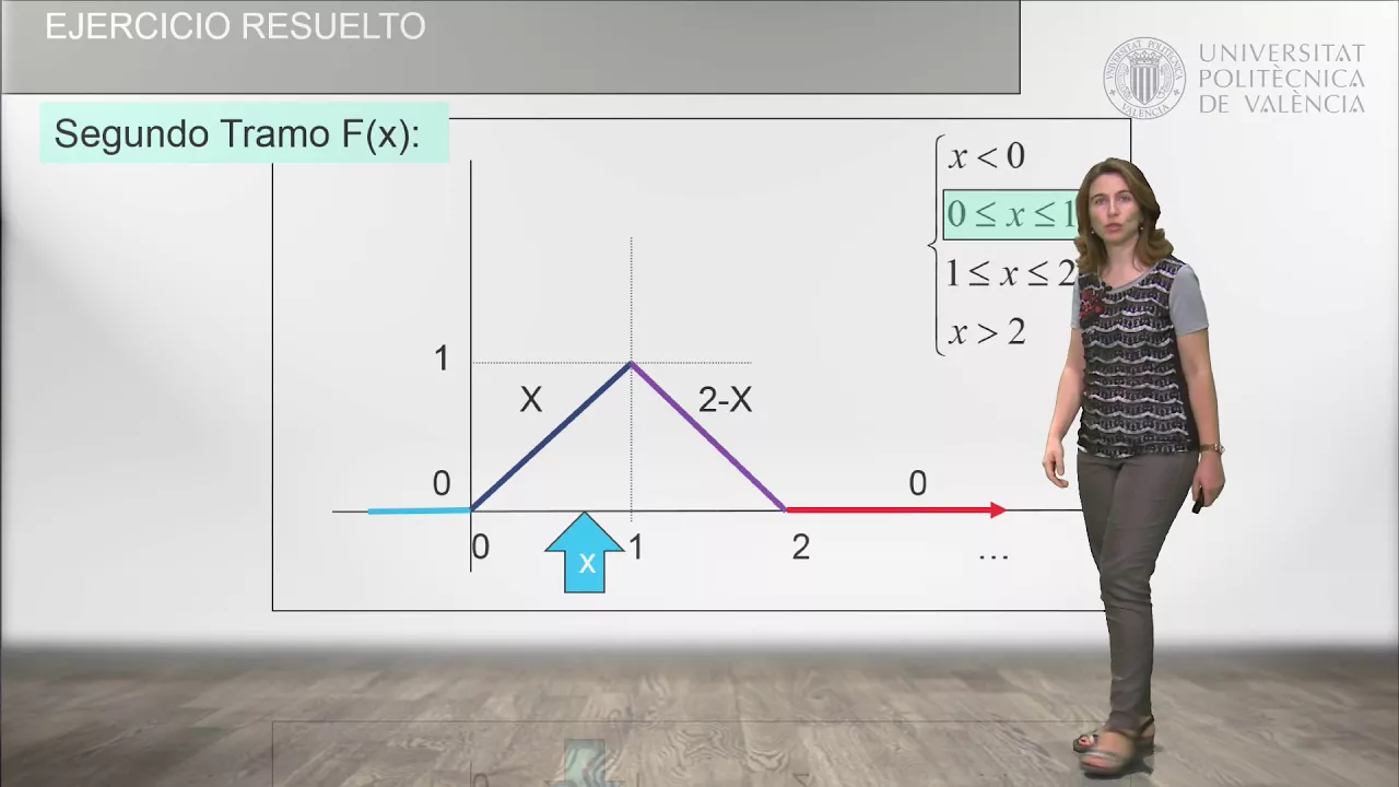











A continuous random variable is defined as a function from the sample space to the real numbers whose range is an uncountable set (typically an interval), and it is characterized by a probability density function (PDF) such that the probability of the variable falling within any interval [a, b] is equal to the integral of the PDF over that interval; unlike discrete random variables, continuous random variables have the property that the probability of taking on any specific exact value is zero, and their PDF must satisfy the normalization condition that the integral over all real numbers equals 1.
Continuous Random Variables and Probability Density Functions Explained
Added:Familiarity with discrete random variables and Probability Mass Functions (PMFs) to contrast with continuous models.
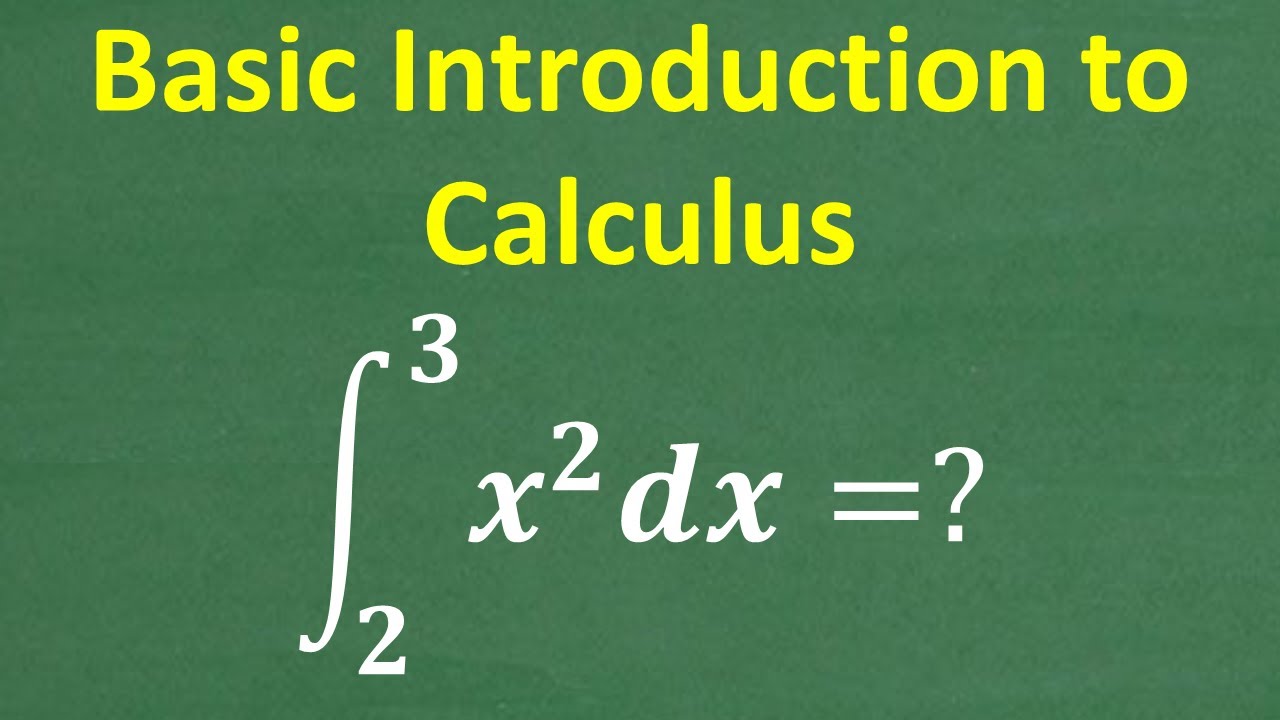
Basic understanding of integral calculus, specifically evaluating definite integrals to find the area under a curve.
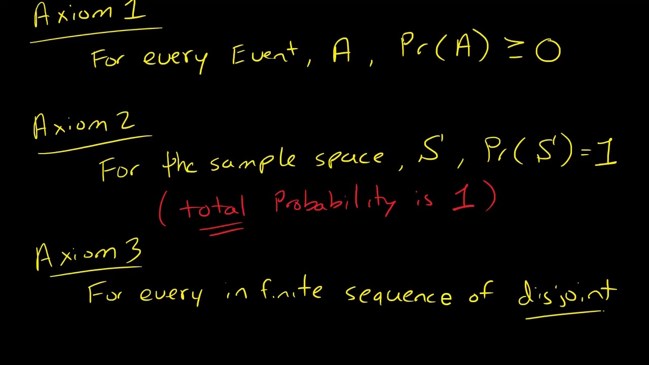
The core axioms of probability, including the concept that the total probability of all outcomes must equal one.
Familiarity with algebraic functions, domain, and range, as well as the concept of limits in mathematics.
Understanding Cumulative Distribution Functions (CDFs) for continuous random variables and their relationship to PDFs.
Calculating expected value (mean), variance, and standard deviation for continuous variables using integration.
Exploring standard continuous probability distributions, such as the Normal (Gaussian), Uniform, and Exponential distributions.
Introduction to joint probability density functions and multivariate continuous random variables.
1.6K views18likes8:03Original Release: 2017-10-31
so we know that a run where ball X is simply a function from the sample space onto the real numbers we see that the random variable is discrete if the range of X is finite or countably infinite there is another important class of random variables called the continuous random variables and those are the topic of this lecture discrete random variables have an Associated probability mass function while continuous random variables will have an associate probability density function and they will be defined differently we defined the discrete random variable from its range unfortunately we cannot do the same thing with the continuous random variable however it is typically the case that the range of a continuous random variable is an interval so the range of a continuous random variable could be something like 0 to 1 meaning that every real number between 0 & 1 is a possible outcome for this random variable the interval may be unbounded so we could have a continuous random variable with the range 0 to infinity or even a range minus infinity to infinity here are some examples of continuous random variables the length of a telephone call in seconds for example where any real number greater than equal to 0 is a possible outcome the second example would be the exact volume of water in a bottle so moving on to the definition of a continuous random variable we say that X is continuous if there is a function f which we will call the probability density function such that any probability such as the probability that the random variable will take a value greater than equal to a and less than equal to B can be evaluated by bring out the integral of f of X from A to B if there exists such a function f such that all probabilities can be found by integrating this function then we say that X is a continuous random variable the function f is called the probability density function abbreviated to PDF for the random variable X the probability density function in turn is determined by the experiment the sample space the probability measure and the exact definition of the random variable however in probability theory it's way more common to specify the probability density function and once we know the PDF of the random variable X we can calculate probabilities simply by evaluating integrals so here is a simple example let's say that the range of my random variable x is between 0 & 1 let's say that my probability density function looks something like this if I want to evaluate the probability that X is between 0.5 and 1 all I need to do is to simply calculate this integral so this area here this area is the same as this probability so it's the integral from 0 to 0.5 to 1 f of X DX where this is my PDF we always make the domain of the PDF equal to the collection of the real numbers and we simply set f of X equal to 0 if X is not in the range of X so in the example above if the range of X was 0 to 1 then f of X is really 0 over here and over here and jumps to whatever a continuous random variable always has an infinite precision since continuous random variables have an infinite precision the probability that X will take a particular value small X must be 0 when we say the probability that X is equal to 0.5 for example we do not mean the probability that X is approximately 0.5 we mean the probability that X is 0.5 with an infinite number of zeros following that 0.5 so that needs to be equal to 0 since the probability of taking on a specific value is 0 the consequence of evaluating probabilities of inequalities will be as follows so this probability in probability that X is greater go to a less than equal to B is the probability that you end up in this interval including a and B while this probability is the probability that you end up in the open interval a through B where a and B are not included well these probabilities must be the same if X is a continuous random variable we can always write this probability as the probability that X is strictly in between a and B plus the probability that X is a plus the probability that X is B since this is 0 and this is 0 these probabilities must be the same you will also get the same result if you have a strict inequality on one side and a non-strict on the other side so for continuous random variables it doesn't make any difference if you used less than sign or less than or equal to sign for any continuous random variable X its probability density function must satisfy one condition and that is when you integrate the probability density function over all real numbers then this must be equal to 1 the integral over all real numbers is equal to the probability that X will take a value Queen minus infinity and infinity and that must be one X will always take a value if the range of X turns out to be something different than minus infinity to infinity for example if I have a range of my random variable X which is just from A to B well in that case it's the integral from A to B f of X DX that must be 1 this will not contradict the property because we can always write the integral from minus infinity to infinity f of X DX as minus infinity to a of f of X DX plus a to B f of X DX plus B to infinity f of X DX if the range of my random variable is from A to B then f of X is 0 outside that interval so that means that it's zero between minus infinity and A and this must be 0 same reason this must be 0 so the integral from minus infinity to infinity will become equal to the integral where we only integrate over the range of X
Up Next
5:01
Probability vs Likelihood: Key Differences in Statistics
@statquest
1.5M views•2018-03-09

4:43
Elliptic Curve Cryptography Explained: ECC, ECDSA, ECDH
@PracticalNetworking
28.5K views•2024-10-21

10:44
Fourier Series Introduction: The Big Idea Explained
@DrTrefor
387K views•2021-05-03

6:00
The Mathematical Impossibility of Accurate World Maps
@Vox
23.3M views•2016-12-02
Related Study Plans & Knowledge Roadmaps
Structured learning paths in Mathematics
mathematics
Tensor Calculus: Vectors to Riemann Curvature
01Mathematical Foundations: Linear Algebra & Calculus
02Covectors, Dual Spaces, and Tensor Basics
03The Metric Tensor and Index Gymnastics
+ 2 more learning modules
40h5 modules
Explore Roadmap
mathematics
Gödel's Incompleteness: Logic, Proofs & Limits
01Introduction to Formal Systems & Hilbert's Dream
02Set Theory, Cardinality, and Cantor's Diagonal Argument
03Arithmetization and Gödel Numbering
+ 2 more learning modules
14h5 modules
Explore Roadmap
mathematics
Galois Theory: Fields, Groups & Solvability
01Foundations of Abstract Algebra: Groups & Fields
02Polynomials & Field Extensions
03Splitting Fields & Symmetries
+ 2 more learning modules
24h5 modules
Explore Roadmap
mathematics
Non-Euclidean Geometry: Models & Geodesics
01Euclid's Fifth Postulate and the Birth of New Geometries
02Hyperbolic Space and the Poincaré Disk Model
03Geodesics: Defining Straight Lines in Curved Spaces
+ 2 more learning modules
15h5 modules
Explore Roadmap