

![Mrunal's [Win21CSP] Economy Pillar 4C - GDP, Inflation, Unemployment | By Mrunal Patel #UPSC](https://i.ytimg.com/vi_webp/xdXu6Mvspes/maxresdefault.webp)





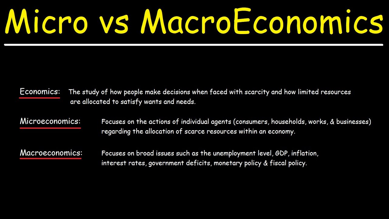
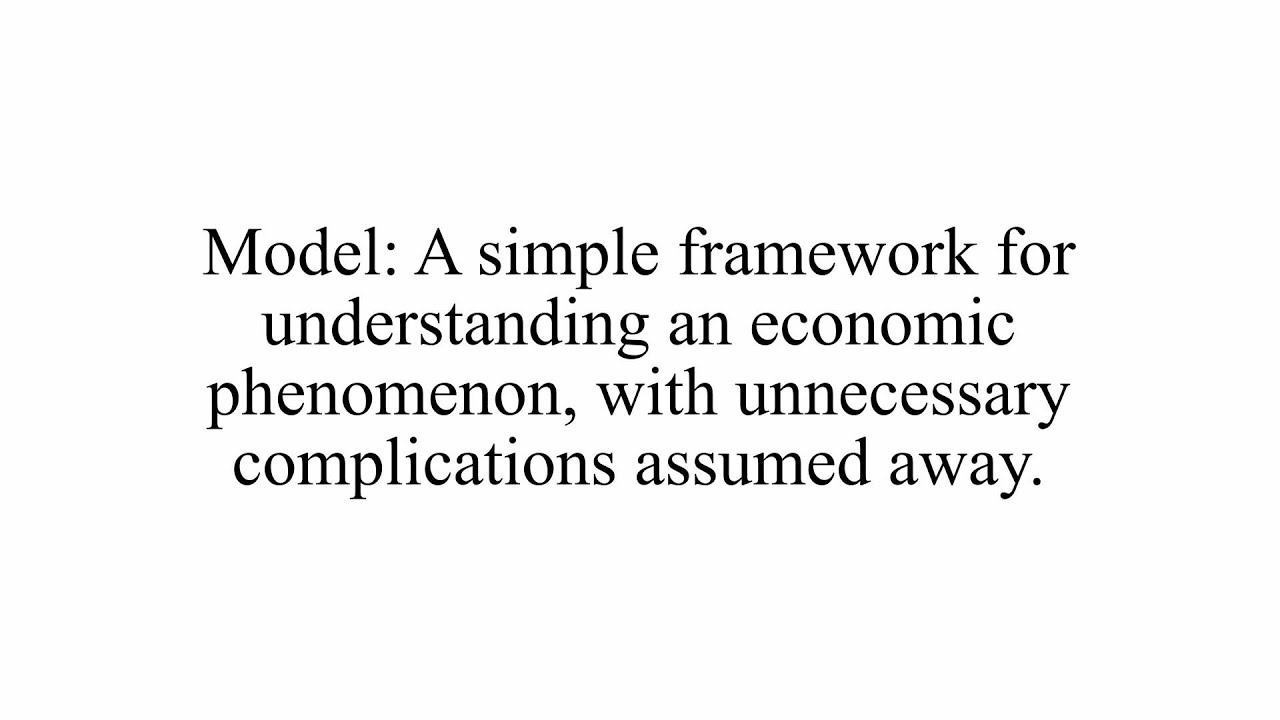







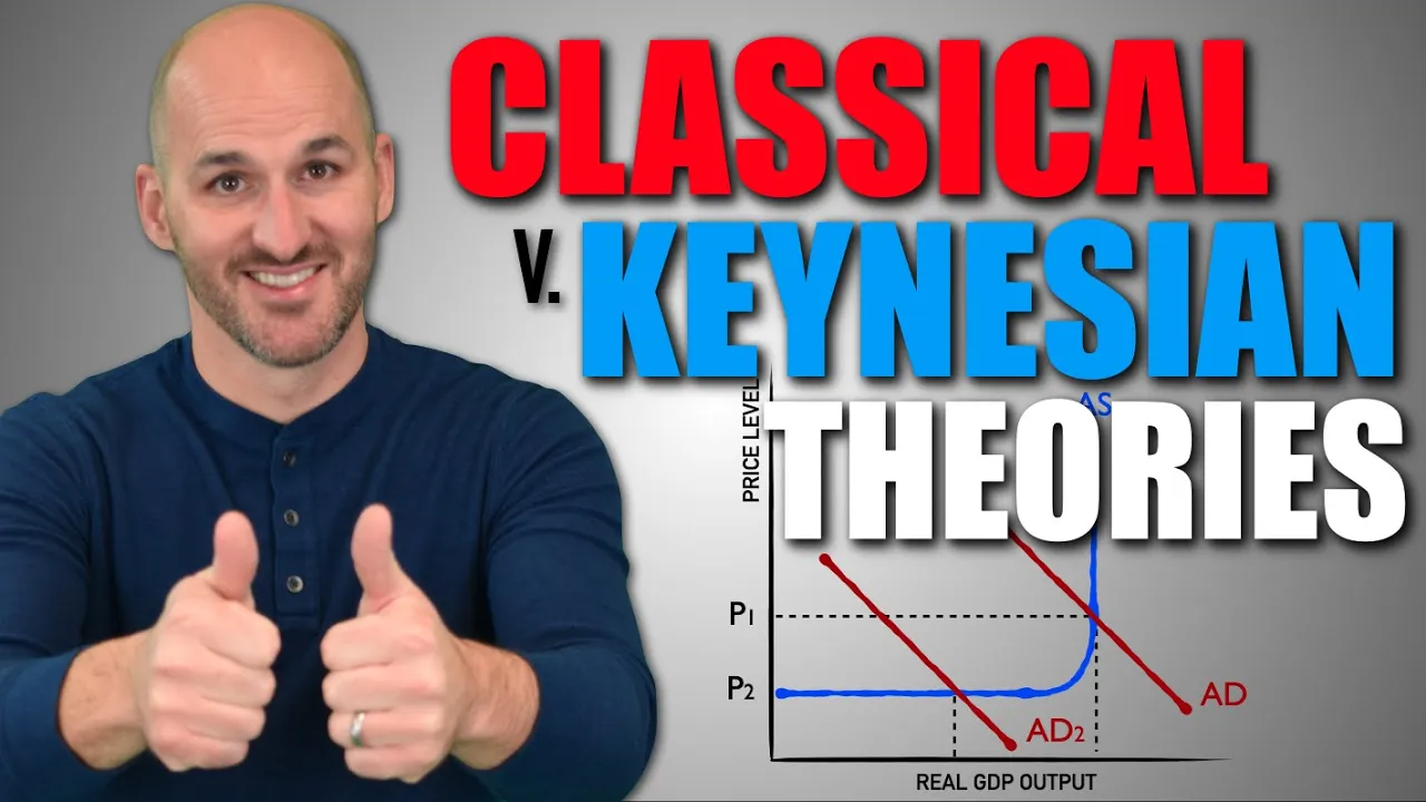



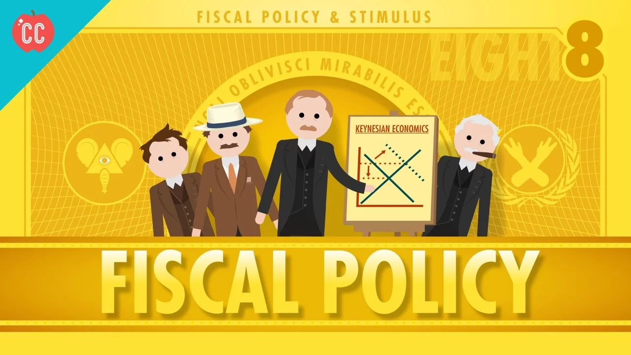
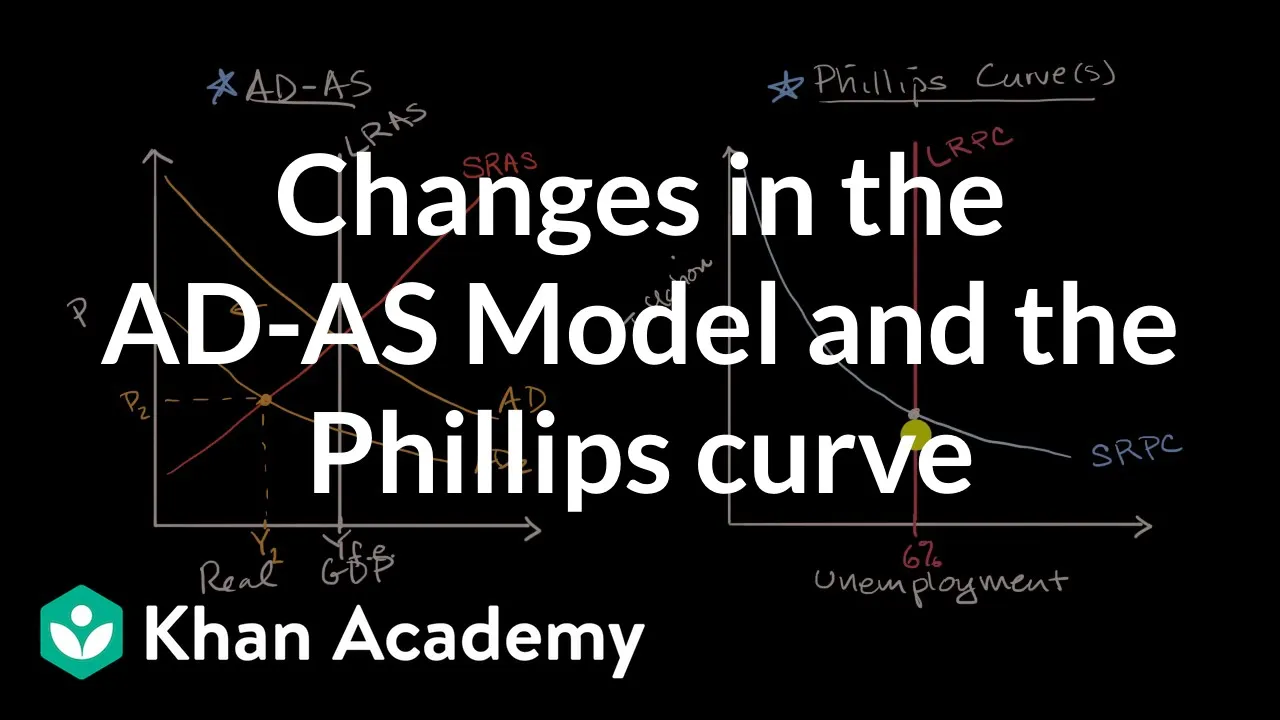
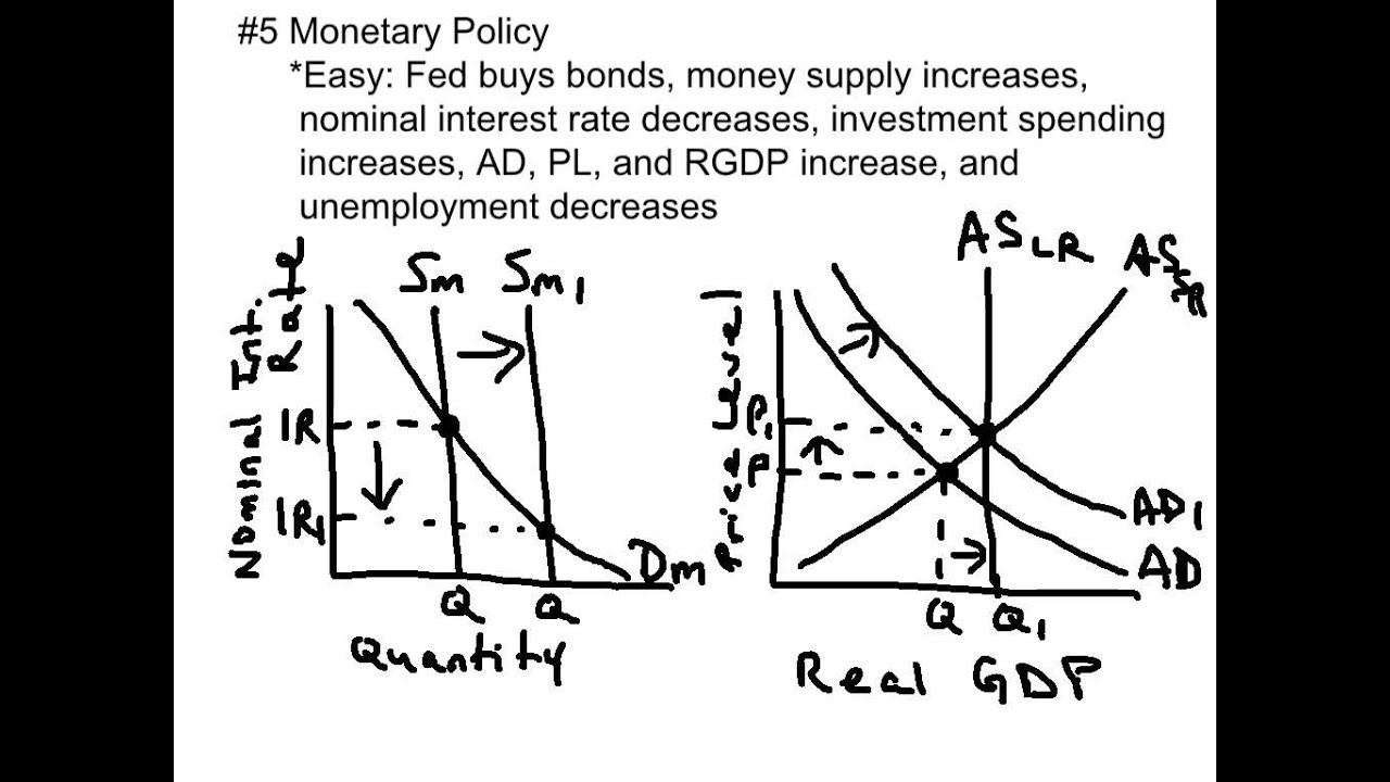






The Aggregate Demand-Aggregate Supply (AD-AS) model explains economic fluctuations through two curves: the downward-sloping AD curve, which shows the quantity of goods and services demanded at different price levels (due to wealth, interest rate, and exchange rate effects), and the short-run upward-sloping SRAS curve (explaining sticky wages, sticky prices, or misperceptions) versus the long-run vertical LRAS curve (determined by labor, capital, natural resources, and technology). Economic fluctuations occur when AD or SRAS shifts, causing deviations from the natural rate of output; in the short run, output and unemployment move inversely, but in the long run, the economy self-corrects back to full employment through adjustments in expectations, wages, and prices.
Aggregate Demand and Aggregate Supply: Macroeconomic Model
Added:okay and down the stretch we come with aggregate demand and aggregate supply this is perhaps the most important of the macroeconomic chapters it develops the model of aggregate demand and aggregate supply is a paradigm that is widely used by many economists policy makers journalists and business people mastering this chapter will give you much insights into how the world really works and it will make the following two chapters of which we're only really covering one in this particular course easier to learn uh most of you will find this to be one of the more challenging chapters in The Textbook however much of the material here should be somewhat familiar from the previous chapters such as the classical dichotomy um the relationship between investment and interest rates a relationship between net exports and the exchange rate this chapter bring to brings together much of the of this familiar material in a new context an aggregate context which allows us to address new and important questions such as what causes recessions and what can policy makers do to alleviate recessions so very quickly in this chapter we'll look for the answers to the to these following questions what are economic fluctuations what are their characteristics how does the model of aggregate demand and aggregate supply explain economic fluctuations how do aggregate demand U curve what why is aggregate demand curve slope downward and what shifts the aggregate demand curve what is the slope of the aggregate supply curve in the short run in the long run what are what shifts the aggregate supply curves so as an introduction over the long run real GDP Grows by about 3% on uh per year on average in the short run GDP fluctuates around this trend so on average it grows about 3% but it's going to fluctuate up and down around that Trend what you want to see is at least a minimum average growth of 3% in recessions those are periods of falling real incomes and Rising unemployment no bueno right depressions are severe recessions which are very rare the short run economic fluctuations are also called are often called I should say business Cycles things fluctuate with the business cycle there are three facts about economic fluctuations that you need to know Fact one is economic fluctuations are irregular and unpredictable um you can see here us real GDP in billions $29 and the Shaded um bars are recessions so we have a lot lot more little recessions um an extended recession would be a depression so these are the little recessions that we've had Fact Two um actually back to F Fact one for a second here economic fluctuations are irregular and unpredictable recessions represented by the Shaded bars here are different um they have different durations and do not occur with any regularity hence the common term business cycle is a bit misleading because as a cycle implies there's something more regular and predictable these are unpredictable and irregular now um Fact Two is that most macroeconomic quantities fluctuate together so what we're seeing here in the graph is investment spending in billions and $29 now I should point out here that investment Falls during each recession this is true of other variables as well when the economy is in recession incomes fall consumer spendings consumer spending Falls profits fall and many stock prices fall tax revenue Falls causing a budget deficit to rise and spending on Imports Falls causing the trade mark uh trade deficit to shrink okay so a lot of not great stuff happens during recessions third fact is output Falls unemployment Rises you can see the unemployment rate here rise when we get into the Shaded bars it's is the unemployment rate um and the percent of the labor force during each recession the unemployment rate Rises when firms cut back on production they don't need as many workers similarly uh during expansions we can see that an unemployment rate falling okay as firms increase their output they need more workers now as a continuation of the introduction explaining these fluctuations is difficult and the theory of economic fluctuations is controversial most economists use the model of aggregate demand aggregate supply to study fluctuations overall fluctuations in the economy the model of aggregate demand and aggregate supply differs from the classical economic theories economists used to explain the long run now classical economics as a recap as what they use to explain the long run and the previous chapters have been based on classical economics especially the classical dichotomy dichotomy just means two parts the separation of variables into two groups we separate them into real and nominal group um real is quantities and relative prices uh real quantities we just uh finished up a chapter talking about real variables it' be the actual physical units and then um prior to that when we talked about Finance we talked about relative prices real prices and before that real GDP means GDP accounting for inflation prices accounting for inflation so that's real that's one half of the D dichotomy and then we have nominal okay measured in terms of money without regard to things like inflation so today's nominal price of gasoline is say is $2 uh today's nominal interest rate is x% now we also have discussed the neutrality of money which is changes in the money supply affect nominal but not real variables it doesn't change the the real GDP because we account for inflation so that's the change in prices um which would change the value of money we increased the money supply right so the neutrality of money um you need to remember um changes in the money Supply affect nominal I.E prices but not real variables I.E fisical units so um the classical economy in the neutrality money pretty straightforward coming out of the last chapter that we covered looking at uh monetary policy and inflation now most economists believe the classical Theory describes the world in the long run but not in the short run in the short run changes in nominal variables like the money supply or P can or prices can affect real variables like output y or the uh Ur rate or unemployment rate to study the short run we use a new model it's the model of aggregate demand and aggregate supply um we have two axes here of course price on the vertical axes and Y here be real GDP the quantity of output on the horizontal axis we have the short run aggregate supply uh curve here short run aggregate supply briefed here and then we have aggregate demand all demand put together and then short run aggregate Supply um very similar to what you would see traditional supply and demand um models here the model determines the equilibrium price and the equilibrium output we have equilibrium here we have our equilibrium price and our equilibrium output um as in previous chapters eqm is short for equilibrium now um the aggregate demand curve ad here uh the ad curve the aggregate demand curve shows the quantity of goods of all emphasis on all goods and services demanded in the economy at any given price level okay um just remember gns stands for goods and services so the aggregate demand curve is shows the quantity of all goods and services demanded in the economy at any given price level so why the aggregate demand curve slopes downward well if you remember from GDP y equals c plus I plus G Plus net exports um consumption plus investment plus government spending plus net exports we assume G is fixed by government policy so they're going to spend what they they have spent um based on some government policy and to understand the slope of um aggregate demand we must determine how the change in price affects consumption investment and net exports well obviously prices go up you buy less so consumption is going down um price of uh interest rate as a price goes goes up you may want to invest more so you're spending Less on output and uh net exports if the value of a US dollar is higher you may buy more Imports if it's you against in an economy where it buys more or if it's lower you might buy it less so th the aggregate demand curve slopes downward now suppose let's look at the wealth effect let's look at p and C so prices and consumption suppose prices rise so suppose P Rises the dollars people the dollars people Hold by fewer goods and services so real wealth is lower okay real wealth is lower have less buying power people feel poorer um as a result consumption Falls so the wealth effect concerns the impact of the price or or excuse me the change in price on wealth and not income when prices fall um we are implicitly assuming that people's real incomes are unchanged which is a safe assumption because incomes are pretty sticky it takes a little while for incomes to adjust to Rising prices and we are only considering the impact of the change in real wealth on their consumption spending so we're just looking at consumption here now let's look at the interest rate effect of p&i so suppose prices rise again okay um we're buying goods and services requires more dollars to get these dollars people sell bonds or other assets that cash them in to get more dollars to buy this drives up interest rates okay interest rates rise because less people are investing thus um investment Falls recall investment depends negatively on interest rates so they have a negative correlation one goes up the other goes down again we're holding real income and everything else constant here at this point some of you may not understand why an increase in household demand for bonds causes interest rates to fall if you wish um just hold on to that actually what I meant to say just hold on to that we're actually going to explain that a little bit more when we get to the next chapter talking about liquidity preference Theory um but uh just hold tight and just know that investment Falls as price Rises as prices go down investment increases okay now the exchange rate effect let's look at price and net exports suppose price Rises okay the US interest rates rise and the in this is called the interest rate effect foreign investors desire more us bonds uh because they're paying at a higher rate higher prices um higher demand for money in the foreign exchange money um exchange market results and the US exchange rate appreciates so US exports become more expensive to people abroad and imports cheaper for us residents more powerful dollar means our prices are higher for people outside of the economy makes it harder for them to buyer Goods a more powerful dollar also means that you can buy more of their goods so what's going to happen is Imports are going to rise and exports are going to fall and that's going to affect net exports and that net exports is going to fall so again the exchange rate effect here Works in reverse a decrease in price causes interest rate and exchange rates to fall which increases net exports now let's look at the slope of the aggregate demand curve again as a summary an increase in price reduces the quantity of goods and services demanded because the wealth effect consumption Falls the interest rate effect investment Falls and the exchange rate net exports Falls so an increase in price reduces the quantity of goods and services demanded note that the red arrow is not equal to the fall and C okay so they're color coordinated here you see the red arrow um it is not not uh the the red ER is not equal to the fall in consumption but rather to the fall in demand due to the fall in consumption so demand is falling the difference is due to the Keynesian multiplier which is initial fall in consumption causes a fall in output which causes a further but smaller fall in consumption now don't worry that word salad won't you won't be tested on I'm just was trying to give you a little bit of the meat um all of this CES a further but smaller fall and output and so forth so it may not um don't worry about I just wanted you to know that the reason why it's smaller is the Keynesian multiplier it's not like something that I'm going to test you on at at this particular chapter but just wanted you to to note that there's a decrease in the wealth effect C Falls is coordinated there in red the interest rate um um effect causes investment to fall and then the exchange rate um causes net exports to fall more Val a dollar we buying more Goods overseas because we can get more of those and people are buying less of ours because it's more expensive to them now why the aggregate demand curve might shift any event that changes consumption investment government spending and net exports except for a change in price will shift the aggregate demand curve if you recall back in chapter four changes in prices are just movement along the curve any event that changes cig or NX so consumption investment government spending or net exports will uh outside of a change in price will shift the demand curve as we see here we're moving from aggregate demand curve one to aggregate demand curve two so it's really not that much unlike what we did way back in chapter four and the demand curve shifting is just we're calling aggregate demand curve an example here would be a stock market boom makes households feel wealthier consumption Rises and The aggregate demand curve shifts right so a change in P won't shift the aggregate demand curve but a but will cause um a move movement along the aggregate demand curve so why the aggregate demand curve might shift um changes in C stock market boom or crash up or down um preferences like uh consumption or saving tradeoff your preferences for consumption versus trade versus saving do you want to save more do you want to consume more tax hikes and tax cuts tax hikes you got less money to consume Cuts you get a little nice check in the mail and you can go out and spend it changes in investment um think like uh firms buy new computers equipment or factories changes in their expectation can affect their um investment if they're having more op optimal optimism in terms of their Outlook um they might spend some more money in investment if they are pretty pessimistic they're not going to invest as much today in terms of firms uh interest rates and monetary policy can affect how much you invest um remember the uh interest rate is nothing more than the price that the bank pays you for putting money in the bank so you may not invest in things if you're not getting a higher price to put your money in the bank or invest in some sort of stock Bond or um annuity so um and interest rate can affect your behavior there and then the investment tax credit or any other tax incentive so if the government gives you some sort of big uh tax credit um on your income taxes for making some sort of investment it's an enticement to invest but if they don't do that that could be a dis incentive to invest okay now again why uh the aggregate demand curve might shift changes in government spending federal spending I.E defense if we had to uh for example defense if we had to uh enter another war or something that would certainly affect um federal spending if we end a war that would affect federal spending so state and local government spending let say things like roads and schools that obviously affects government spending which affects aggregate demand may cause it to shift and then changes in net export booms recessions um in countries that buy or exports okay so if you have a boom in a country that loves to buy a bunch of American Goods they're going to buy more American Goods if they have a recession they're going to buy less American Goods which affects our our ratio of net exports U there can also be appreciation depreciation resulting from International speculation in Foreign Exchange Market so what's going on in the other markets can affect the expectation and the consumption um of imports from the US okay let's take a quick look at Active Learning activity the aggregate demand curve um what happens to the aggregate demand curve in each of the following scenarios let's take a look at a b c and d uh aggregate demand curve what's it going to do a 10-year-old investment tax credit expires might affect investment might cause investment to decrease uh B the US exchange rate Falls okay perhaps our money isn't worth as much on the World Market perhaps um if it's not we'd be more inra attractive price-wise for other countries want to buy our Goods because our stuff's technically more affordable um the fall in the prices increased the real value of consumer wealth so if prices go down you can buy more things with the money you already have so you in turn have more consumer wealth and that could affect consumption State Governors replace their sales taxes with new taxes on interest dividends and capital that's going to affect how much you uh choose to invest that would be a deterrent I would say um a 10-year-old investment tax credit expires that's the first one investment Falls and aggregate demand shifts left okay just as we osed um the US exchange rate Falls uh net exports rise we're going to we're going to export more because our stuff's more affordable because our dollar is not as powerful or as valuable I should say aggregate demand curve shifts to the right a fall in prices increases the real value of consumer wealth okay um we are going to have a wealth effect we're going to move down along the demand curve that's movement along the demand curve it's not a shift okay so we get two shifts got one left one right we got moving along the demand curve um state governments replace sales taxes with new taxes on interest dividends and and um and capital gains so people are going to it's going to affect that that saving and consumption ratio um people are going to save less so that means they're probably consuming more and the aggregate demand curve shifts right so that's an interesting play on that now aggregate supply C cures as the aggregate supply curve shows the total quantity of goods and services firms produce and sell at any given price level now aggregate supply is upward sloping in the short run and vertical in the long run so we have two aggregate supply curves here uh the traditional supply curve that you're used to short run aggregate supply curve is represented here in this blue and then in the long run we're just fixed in the long run we're producing everything we can produce so it's fixed on some level of output and the long run aggregate supply curve is vertical now uh the long run average um long run uh aggregate supply curve l r s uh looking here the vertical fixed long run AGG aggregate supply curve the um natural rate of output which is y subscript n natural rate of output remember Y is output and n is the natural rate is the amount of output the economy produces when unemployment is at its natural rate okay in the long run the people who are unemployed are going be going to be unemployed that's your natural rate um recall back from the unemployment chapter YN is also called the potential output or full employment output so if all the people who don't want a job don't have one in the long run um you have a natural rate of unemployment we just have those people that are constantly in transition we're employing everyone we possibly could employ in that point in the long run what would our output be it would be right here this is our long run aggregate supply right here vertically fixed on some level of output boom now why is the long run average supply curve or aggregate supply curve I should say apologize for keep saying average long run aggregate supply curve is vertical so your natural rate of output is determined by the economy stocks of Labor Capital natural resources and of course the level of technology that we talked about uh back when we covered GDP an increase in price does not affect any of these so it does not affect the natural um output in the long run it's the classical dichotomy again all right you're producing a certain amount of goods and services that is real goods and services price can go up but it can't affect in the long run what you can produce because that all depends on the economy stocks of Labor Capital natural resources in the long run you're doing what you can do and and at the highest rate you can do it so it's fixed um in any event uh any event that changes any determin of the national rate of unemployment in the long run will shift the long run aggregate supply curve U say for example immigration increases that's increased labor in the market uh causing output to rise so if you have more of an input say more of Labor capital or natural resources that something new is discovered it can shift the long run average supply curve to the right now changes in labor or natural rate of unemployment um things that can change labor are the natural rate of unemployment we have immigration of new workers coming in Baby Boomers retire certainly affects the supply of labor on the market if everybody this big group of people which we're going to see start to retire they're not working it this huge decrease in the number of people in the labor Supply um government policies could reduce the natural unemployment rate so there could be some sort of policy that uh entices more people into the market could be some policy that uh discourages more workers and and your natural rate of unemployment changes now changes capital or um or knowledge here H you can have investments in factories and Equipment more people get college degrees um uh capital is K and then I said knowledge what I mean here is human capital so more people get college degrees you're here in school building human capital right now uh or factories heaven forbid gets destroyed by a hurricane or some other natural disaster that certainly is going to affect the long run AG um aggregate supply curve so why the long run aggregate supply curve my ship continue there could be changes in natural resources discovery of new mineral deposits say they find a new um source of crude oil somewhere reduction in the supply of imported oil okay so uh you discover new mineral deposits that's certainly going to reduce your supply of imported oil uh changing weather patter changing weather patterns that can affect agricultural production say the amount of corn or something that we can produce the amount of wheat that we can produce um so on and so forth changes in technology uh we can have productivity improvements from techn technological uh progress we have some new discovery that allows us to do something much more quickly than we used to do so we can use aggregate demand and aggregate supply to depict long run growth and inflation okay over the long run techn technological progress shifts the long run average u a aggregate I'll get it down one of these days long run aggregate supply to the right okay we have 1990 2000 2010 what's happened uh we have technological progress we we learn new things and all of a sudden our long run average supply curve we can produce more and more output you keep growing to the right now and the growth in the money supply shifts the aggre demand to the right give people more dollars they're going to demand more things okay result there's ongoing inflation and growth in output Okay so we've got prices going up and up and up there's ongoing inflation um some of this is tied to obviously the increase in things that we can buy some of this is tied to printing too much money and perhaps prices um increase over time quantity theory of money from the previous chapter um but as you can see over time productivity goes up prices keep going up now let's take a look at the short run aggregate supply curve the short run aggregate supply curve is upward sloping so over the period of one to two years an increase in price causes an increase in the quantity of goods and services supplied so you see we move here um we have that increase in output we have an increase in prices so that's an inflation over a period of one to two years an increase in prices causes an increase in the quantity of goods and services Supply it's better of an En enticement for additional production from y1 to Y2 so why the slope of the short run aggregate supply curve matters if aggregate supply in the short run at least is vertical fluctuations in aggregate demand do not cause fluctuation in output or unemployment so if it was just fixed straight up and down uh there's going to be no increases in employment so short run accur supply curve is is sloped so we can see those increases in output and if you're going to Output more as a producer you're going to have to hire more people so that's the fluctuations in employment and output if the aggregate supply um curve slopes up then shifts and aggregate demand do affect output and employment as you can see here in long run it did not affect output it's stuck right here in the short run um if it's if it's slope like this you see short run Ag Supply shifts do affect the amount of output that we have and thus you know it affects employment now there are three theories of short-run aggregate supply in each there's some type of Market imperfection it's an imperfect world after all the result is output deviates from its natural rate of output when the actual price levels deviate from the price level people expected so a lot of expectations here each of these theories provides a reason why the aggate supply curve might have a positive slope in the short run okay let me caution you here these three theories of short run aggate Supply it's a longer chapter but I really want you to know that it would be most helpful if you carefully read this section in the chapter okay carefully read this section in this chapter now first one is the sticky wage Theory you've heard me reference this in class A few times um imperfection nominal wages are sticky in the short run you can't really just go in and get a raise anytime you want they just sluggishly okay this is due to labor contract and social norms um social Norm is just kind of what's acceptable and your boss is not going to think it's acceptable for you to continuously walk in and get multiple raises per year now firms and workers set the nominal wage in advance um based on the price equilibrium so the price level they expect to Prevail so or excuse me not price equilibrium this is their expected price the E is their expected so you expect something to you know be at a certain price that affects what a firm uh wants to pay you it also expects whatever your expectations are what you expect for a nominal wage your set salary okay so the firm might expect you um to need to earn one level and then you might have a different set of expectations and there's a bit of a negotiation that goes on between you so the price level um that one expects is what prevails what you expect to be to earning and what the company expects to have to pay you perhaps you meet in the middle now continue with the sticky wage theory if the actual nominal price is greater than the price that is expected revenue is higher higher but labor cost is not production is more profitable okay you're getting a higher nominal price and um so they can increase output and employment hence at the higher price uh the higher price causes higher output so the short run average curve slopes upward so if p is greater than price expected this means that if the actual price level turns out to be higher than the price um fir level firms had expected they'll have higher revenue and want to increase their output and hire more people now here's the imperfection um here's another imperfection the second one as it deals with the sticky price Theory many prices are sticky in the short run due to the menu cost that we covered in the last chapter um it's kind of expensive to just continuously increase your costs I.E a restaurant changing its menu all the time the cost which is the menu costs are simply those cost of adjusting prices now examples in include cost of printing new menus the time required to change price tags Etc firms set sticky prices in advance based on what they expect prices to be their price expectations okay to try to minimize menu cost now suppose the FED increases the money supply unexpected in the long run prices will rise because it'll take more dollars to buy things you want in the short run though firms without menu costs can raise their prices immediately firms with more menu costs wait to raise prices because they don't want to incur those transaction costs of increasing their their their cost on their menus for example um meanwhile their prices are relatively low which increases demand for their products so they the menu cost deters them from increasing their prices which actually makes them more attractive in the market so they increase output and employment they get real busy hence the higher the price is a higher price is associated with a higher output so the short run average um supply curve slopes upward now the third thing we're going to look at here is the misperceptions theory so we did two things with sticky price Theory and now we're going to look at the misperceptions theory here's the imperfection though firms May confuse changes in price with changes in relative price of the the products they sell relative is real price if prices rise above um the price expected a firm sees its price rise before realizing all the prices are rising The Firm May believe that its relative prices rising and may increase output in employment so an increase in price can cause an increase in output making the short run average uh aggregate supply curve there we go again short run aggregate supply curve upward sloping okay of the three theories this one seems least plausible I think the other two um are part of what's really going on in combination but this one seems the least plausible firms certainly have a strong incentive to not make a mistake on a general price increase for a relative price increase and information about price level is Costless and available with only a short lag especially the CPI you can look at that which is published monthly you can see that monthly so every four weeks you can look at C C and we'll see what's going on with inflation and adjust your prices accordingly so in CPI is also very widely reported in the moment it comes out so it's not like it's hard to find so I don't know so much about the misperceptions theory I subscribe very heavily to the sticky price Theory and the sticky sticky wage um which is the price you charge for your labor and the sticky price which is what people charge or businesses charge people to consume it so I tend to Camp more on sticky wage and sticky price than I do the misperception Theory just my normative statement so what all what the three theories have in common in all three uh theories output deviates from the natural rate of output when the price deviates from the expected price so you think about it it actually makes sense you expect output to be on some some level just set on some level and you expect prices to be on some level wouldn't those sort of go hand in hand you expect the price and an output to be similar if you expect price to be higher you expect output to be higher to chase that price well if output actual output and price deviates from those things um all three of those theories that we just covered have that in common again um y equals uh the output equals the natural rate of output in Long Run plus a which is you would think greater than zero which measures how much output responds to unexpected changes in price and then you have the actual price level nominal and the expected price level okay economists debate which one of these theories is correct it's possible that each of them can contain some element of Truth just like I said I thought it was more of a combination between sticky wages and sticky prices but for our purposes here the similarities between these theories are more important than their differences it's all why that makes that short run aggregate supply curve slope upwards all three imply that output deviates from the long run level which is the natural rate of output when the price level deviates um from the level people had expected that price expected so so it's all expectations versus what happens and how that affects output now um the preceding slide introduces the equation of aggregate supply that shows how output deviates from Full Employment when the actual price level is different from the expected this slide illustrates these Concepts using a graph so when the price equals what the expected price would be the output is going to is going to equal the expected output when the um price that actually occurs is less than the price that you expected then the um actual output is going to be less than what you would think the natural rate of um output would be and then lastly when the price is greater than what you expected prices to be your output is going to be greater than what you expected output to be okay pretty pretty straightforward so um when the price is greater than what you expected here's the price that you expected the expected price level and that's where it hits the short run aggregate supply curve um when the price is greater than what you expected then the output is going to be greater than what you expected okay it's going to be over here right it's going to hit the line here and come here which is greater than the natural rate of output okay and when the p is uh when the actual price p is less than the price expected okay you're going to hit the short run aggregate supply curve over here and output is going to be less than your natural rate of output okay if it hits if it hits where you expect it's going to produce what you expect if it's below it's going to be below it's above it's going to be above okay now now shter aggregate supply and long R and aggregate supply the imperfections in these theories are temporary over time sticky wages and prices become flexible okay over time you can argue for a raise over time firm can change their prices now in misperceptions over time can be corrected in the long run the price expect the expected price equals the nominal price and the aggregate supply curve is vertical it's fixed on some um some production based on some level of output based on our production capabilities the technology the labor and the capital that we have available in the long run is fixed so put it all together uh notice that when the price levels uh equal the expected price level output is equal to its long run value okay the natural rate of output um you know it's equal to its long run value which is the natural rate of output now this can be interpreted U by saying in the short run people may be fooled about price level or they may be locked into wages and PR or prices that were set before they knew what the price level would actually be hence in the short run price May differ from the expected price but in the long run expectations catch up to reality price starts to to equal what you would have expected short run there may be some variations therefore in the long run output starts to equal the natural rate of output as in the classical model so it's just in the short run there's some deviations there thus our theory of economic fluctuations is basically the classical model which we studied for several chapters this semester augmented with some kind of Market imperfection such such as sticky wages or sticky prices the impact of the market imperfection occurs only in the short run so the long run behavior of our model is classical all right it's just in the short run this is that thing we sitting in classes like well my pay doesn't variate as quickly as the price that's exactly right that's why the classical model doesn't necessarily explain things in the short run your pay does not it's sticky it has to take time in the long run you can adjust either by getting your your current firm to pay you more or making a move to another firm that values you more or getting some more skills that can get you a high higher pay so in the long run all those things are possible in the short run they're sticky otherwise we'd all run out right now and get everything we wanted paywise now why might the short run aggregate supply curve um shift everything that shifts long run aggregate supply shifts short run aggregate supply too so also price uh the expected price shifts aggregate supply and then if uh if expected price Rises workers in firms set set higher wages okay at each price production is less profitable and output Falls as the short run supply curve shifts left that's pretty natural shift that we have been covering since um chapter four really we talked about supply and demand we're just talking about long run and short run here so we know short run aggre Supply can shift left um that will affect um if you had a demand aggregate demand curve here that will affect your output but in the long run prices do increase and the output will be fixed so long run equilibrium in the longer in equilibrium the price expected equals the the current price and the output currently equals the natural rate of output and unemployment is at its natural rate in the long run the thing is is we're always in a new short run okay uh 10 years ago we would have said today was the long run for sure but the thing is today is our short run for 10 years now okay or a year from now so um short run aggregate supply is going to look like your traditional supply curve you see here aggregate demands pretty much always going to look like your um your your traditional demand curve we're just talking about aggregate here when we're talking when we're talking aggregate we got to talk short run and long run in the long run it's all vertical fixed basically on uh our current technology level what we can produce our label labor labor level what we can produce currently and our Capital level what we can produce currently that's going to be some fixed amount of output now e economic fluctuations can be caused by events that shift the aggregate demand Andor aggregate supply Cur they can both move so think again chapter four supply and demand curves can move there are four steps to analyzing e economic um fluctuations the first is determine whether the EV the event shifts aggregate demand or aggregate supply next we need to determine whether the curve shifts left or right is it an increase or decrease and we need to use the aggregate de aggregate demand aggregate supply diagram to see how the shift changes output and price in the short run because remember we're talking two different things what's it going to do in the short run versus the long run then lastly fourth uh we can use the aggregate demand and aggregate supply diagram to see how the economy moves from a new short run equilibrium into the longer run equilibrium you know when things are fixed and we have a vertical supply curve this four-step approach is based on the three-step approach we used in chapter four to analyze changes in basic supply and demand model or basic sply demand models it's chapter four all over we're just putting everything every good and service all together so the effects of um a shift in aggregate demand let's say in the event of the stock market crash okay this affects consumption which is the aggregate demand curve we move from aggregate demand curve one which is blue down to aggregate demand curve two which is red um the short run equilibrium at point B and the price and output are lower and unemployment is higher okay so we move from uh short run a down to point B so we got a decrease in production which implies that unemployment is going be higher if we're not producing as much we don't have to have as many workers and prices actually went down um over time the expected price Falls okay and the short run aggregate supply curve shifts right until the long long run equilibrium is at C okay in the long run our our short run curve is going to to to Pivot pivot pivot until it's um vertical and we're at um Point c um where Y and unemployment are back at initial levels so there's going to be some fluctuations but we have this basic level of growth remember I said GDP typically grows about 3% sometimes we're going to be below it sometimes you're going to be above it sometimes that means if you're below it you're not as productive you have more unemployment if you're more productive you have lower unemployment but chances are we're going to move back to that medium and move back to that um initial area in the long run the results of this exercise apply to any event that shifts aggregate demand to left whether it's a stock market crash a recession abroad or a wave of pessimism and expectations or something something else um the stock market crash reduces consumers wealth in this example which depresses their spending so the aggregate demand curve shifts to left the new short run equilibrium is at point B where price and output are lower hence unemployment's higher you don't need as many workers to produce less now remember fact number three of the economic fluctuations unemployment output move in opposite directions okay so if we have a lower output we're going to have higher unemployment if we have higher um if we have um higher output we're going to have lower unemployment more people put to work here we have higher unemployment low because of lower output so at point B the nominal price is less than the expected price and over time uh the expected price Falls wages fall sticky prices become flexible and fall and the short run average cost curve moves rightward so that's that short run average cost curve moving to the right because well the price expected Falls the wages fall and sticky prices become flexible and fall this process continues until the economy arrives at Point C where GDP and unemployment back at their natural rates and price expected equals price once again now notice that in the absence of policy intervention U the economy self-corrects if you will of course this process takes time and policy makers do not want to wait why because policy makers need to be elected the next six months for SE and they can't wait for the long run at point B policy makers could use fiscal or monetary policy to shift the aggregate demand back to to the right and move the economy back to a typically that's what we try to do we start fooling around with things and sometimes we have unintended effects where we mess up something when the market could have corrected for it itself we lack patience imagine that so it can be artificially done but the Market's going to end up back there at the long run anyway now here's two big aggregate demand shifts uh the first being the Great Depression it lasted from 1929 to 1933 the money supply fell 28% due to problems in the banking system stock prices then fell 90% reducing consumption and investment you think um output fell by 27% and prices fell by 22% okay um the unemployment Rose from 3% of the economy to 25% so one out of four people didn't have a job that's pretty tough two possible causes for the Great Depression was the fall in the money supply and the stock market crash neither would shift the aggregate demand curve left causing price and output to fall and causing unemployment to rise which is exactly what happened the second one the second big aggre demand shift was the World War II boom okay so look how these correspond you had the Great Depression from 29 to 33 and then the World War II boom that came in the late 30s through the mid 1940s um government outlays Rose obviously we're at War we're producing a lot of things from 9.1 billion to 91.3 billion that's a big jump in a 5year period so excuse me uh output Rose by 90% and prices rise by 20% unemployment fell from a Gody 177% down to 1% everybody everybody was working had to you had a bunch of um bunch of people fighting a war overseas and then everybody entered the market stay-at-home moms were producing things they were they were helping build bullets and and and and tanks and all these things so the boom was this boom was clearly caused by surge in government spending I mean it's clear our model predicts an increas in in government spending G would shift aggregate demand ad D to the right causing P which is price and output y to um increasing price and output and reducing unemployment put more people to work you're going to be more productive U prices are going to go up U because government spending is up these uh predictions are consistent with the data so pretty straightforward so we got a we got a boom and we got a bust okay can really shift aggregate demand so let's let's think through an active learning activity working with the model draw an aggregate demand short-run aggregate supply and longr run aggregate supply diagram for the US economy starting in the long run equilibrium and then a boom occurs in Canada use your diagram to determine the short run and long run effects on US GDP and the price level in unemployment so if you want to pause here you can otherwise I'm going right into into it the event in Canada the Boom in Canada all right this affects net exports and that and the ad curve all right so the aggregate demand curve actually shifts okay that it shifts the aggregate demand curve to the right and the short equilibrium at point B where price and output and un is higher price and output is unemploy uh is higher price and output is higher and unemployment is lower because if you're going to do more output you need more workers that's going to take people off unemployment and then over time the price expected rises in the short run um aggre supply curve shifts to the left uh until the long run equilibrium is back at c u output and unemployment are back at their initial levels prices are up so a boom in Canada increases the incomes of cons Canadian consumers in turn their spending Rises some of their spending is on products from the US so their spending increases causes uh spending increases caused US exports to rise this shift in the US aggregate demand curve to uh this shifts the aggregate demand curve to the right the new short run equilibrium is at point B where price and output are higher okay hence unemployment is lower now at point B the nominal price is higher than the price expected okay so um over time the expected price Rises with it wages rise sticky prices become flexible in the long run and rise and the short run average cost curve uh short short run aggregate supply curve I should say apologies short run aggregate supply curve moves leftward for a minute there I was trying to teach you micro and macro um this process continues until the economy arrives at Point C where GDP and unemployment are back at their natural rates and the ex expectations about price have caught up with reality they're higher now let's look at a case study the recession from 2008 to 2009 so from December 2007 to June 2009 real GDP fell by 4.7% doesn't sound like a big fall but that's huge supposed to be growing by 3% each year it fell by 4.7% in that um year and a half all right unemployment Rose from 4.4% in May of 2007 all the way to 10% of um willing enable workers by uh October of 2009 the housing market played a central role in this recession now look at the case Schiller home price index don't worry you have to know what that is it's just a a 20 City Composite Index looking at uh adjustments in um in home prices so home prices went up and up and up and up and up and this is called a bubble see this bubble what happens to Bubbles they pop comes back down to earth so bunch of people bought houses up here and then all of a sudden they were worth this that means you're upside down in your house housing bubble played a central part in the 2008 to 2009 recession now Rising house prices during 2002 to 2006 due to low interest rates and it was very easy to get credit um through subprime borrowers people were giving people bananas loans to buy these houses they couldn't afford government policies also um aimed at increasing home ownership kind of encouraged this type of practice um really uh Clinton towards the end of Bill Clinton towards the end of his um uh tenure as president said the American dream was to own a home um that really kind of shifted policy towards um let's make that possible and it gave a lot of people the ability to own homes that they couldn't otherwise afford so government policies increased home ownership rate then there was the securization of mortgages investment Banks purchased mortgages from lenders and created Securities backed by these mortgages they basically made them a mutual fund and like pile of mortgages as an investment why because the price of houses was going up and people were making so much money doing it they were making Quick Cash when people paying off their loans plus interest they sold these Securities to Banks insurance companies and other investors people became really really leveraged the financial sector became really leveraged and the real estate market which you know is blowing up and about to be a bubble um the mortgage back Securities Perce were perceived as safe since the housing prices would never fall I mean their houses were great Investments everybody let's get into houses well what happens well there were some consequences of the6 the 2009 housing market crash it did crash it was a bubble it burst millions of homeowners were underwater they owed more money than what the house was worth because the prices were no longer up on the bubble they fell down millions of mortgage defaults and foreclosures resulted Banks selling foreclosed houses increased the Surplus and further pushed the downward uh further pushed prices downward so Supply got huge all of a sudden if Supply is huge something's less scarce if it's less scarce it's less valuable um the housing crash badly damaged construction industry as well and they employ a ton of people 2010 unemployment rate was 20.6% in construction versus 99.6% overall that is bananas that's a high rate for any industry um mortgage back Securities became toxic everybody had a ton of toxic Securities they were backed by mortgages there were heavy losses for institutions that purchased them and widespread failures of banks I mean straight up failure Banks going under and other financial institutions were failing as well this sharply rised the unemployment rate and had a falling GDP there less lending less investment less investment less production and on down the rabbit hole we go less production incomes go down GDP comes down healthc care gets worse education gets worse crime goes up all these bad things happen all at once and oh yeah by the way people didn't have jobs so here was the policy response the Federal Reserve reduced the federal funds rate uh Target uh to near zero so Banks can get more money more easily to stay solvent the Federal Reserve purchased a lot of those bad toxic mortgage back Securities and other private loans and basically said okay American people are going to buy this so we can still have an economy um controversial whether or not they should have done that or just let the let the people go Belly Up um the US Treasury injected Capital into banking system gave them some more money think about Monopoly when you ran out of money they they literally gave them more money to increase the bank's liquidity and solvency and hopes of staving off a complete credit crunch where they couldn't loan anything to anybody and we couldn't grow these fiscal policy makers incre also increase government spending and reduced taxes by about eight billion okay increased government spending that puts more money into the economy it's a short run little shot in the arm think of a B12 shot to give the economy a little shot in the arm and then Al also by reducing taxes by 800 billion that put a a check in everyone's mailbox and they went out and bought things in an economy where Merchants restaurants all these people were dying for somebody to come buy something so how do you do that you s them much check problem is you put more money in the economy in the long run money is less valuable and you have big jumps in inflation now let's look at the effects of a shift in short run aggregate supply let's take an event where oil prices rise an increase in cost shifts the short run aggregate supply you can assume the long run aggregate supply are constant the short run aggregate supply shifts left and the short run equilibrium at point B okay short current equilibrium moves from A to B here and the prices are higher and out outp put is lower um so that means unemployment is higher so from point A to point B we have something called stagflation which is a period of falling output and Rising prices when you see this y going down that's output falling and when you see this P going from P1 to P2 that's prices rising when you see output falling and prices rising that by definition is stagflation an increase in oil prices might might also affect the long run average Supply but for Simplicity and to be consistent with the textbook we assume it only affects short run aggregate supply so we're holding aggate Supply Here constant okay theoretically AGG Supply might just Retreat back to this point and then you're at your new long run aggregate supply um but what we're going to do here is illustrate so if you see on the test y decreasing that's decrease in input or decrease in output I should say y natural rate back to Y2 and you see an increase in prices uh yes that's inflation but when it couples with a decrease in output it's called stagflation now uh if policy makers do nothing uh what would happen fourthly is low employment causes wages to fall okay in the short run aggregate supply shifts to the right because people are labor is more affordable okay so companies will say hey well let's Supply more because we can afford more labor until the longer and equilibrium is back at Point a okay or policy makers could use fiscal or monetary policy which is what they're going to do because they're impatient because they're trying to get reelected okay they're not going to wait for the long run in the long run the economy is like trying to adjust the voters aren't happy they don't have a job so they vote for new people so policy makers could make physical and monetary policy in to increase aggregate demand and accommodate for the aggregate supply shift why moves back to the Natural rate of output Y in but p is permanently higher so there's a cost to being impatient okay there is a cost to being impatient and that prices are going to rise okay we stay at this higher price instead of adjusting backwards where we go back to the lower price at a so we're at C versus a the same level of output we get paying higher prices sound familiar should now the 1970s we had oil shocks and their effects this is way before most of my students um knew what was going on uh we had real oil prices uh that increased by 138% from 1973 to 75 from 78 to 80 went 99% CPI you see going up and up and up real GDP actually went down during the initial period went up um over the second period number unemployed H prices go up output goes down unemployment goes up okay the prices real go really go up the unemployment really goes up prices go up unemployment goes up obviously when the prices went up more you had more unemployed when they went up less you still had some unemployed but wasn't near as bad as the before both scenarios were not ideal so the first oil shock occurred in 1973 to 1975 uh oil prices more than doubled in just two years causing the short run aggregate supply to shift leftward as our model predicts the price level Rose GDP fell and unemployment Rose now from 1975 to 1978 oil prices Rose at less um than the rate of inflation the number of unemployed persons fell by about 1.7 million okay real GDP grew by about 16% the economy was self-correcting imagine that letting it correct on their own um but just when things were getting better a second oil shock hit oil prices doubled again and this was do in part by the Revelation uh Revolution I should say in Iran in 1979 Iran used to be much more free than they are now um they had a revolution where um some not so nice guys took over and uh put Sharia law if you will into effect again though as our model predicts short run aggregate supply shifted to the left inflation Rose unemployment increased the table shows that real GDP Rose by 2.9% during this period but remember this was not the annual rate it is a 2.9% uh rate for the entire period so that's not enough for a one year one year increase of 3% this is for like multiple years here so it's substantially lower um or substantially below the long run average growth rate of about 3% per year now this a guy named John Mayor kees he lived from 1883 to 1946 he wrote the general theory of employment interest and money in 1936 he argued that recessions and depressions can result from inadequate demand um policy makers should shift he he argued that policymakers should try to shift aggregate demand I would argue that this makes prices go up and up and up um the famous critique of he had a famous critique of classical theory that uh the long run is misleading guide to current affairs in the long run we all dead economists set themselves uh too easy to to the useless T to to useless a task if their tempestuous Seasons um they can only tell us when the storm is long p and the ocean will be flat basically he was pointing out the fact that classical economists are much better in the um looking in the rearview mirror than they are forecasting ahead and that we should put our hands on the steering wheel and try to drive the economy as best we can through monetary policy much of the theory in this chapter and the one that that follows originates in the work of of canes now this slide reproduces his famous critique of the long run focus of classical microeconomists what's what's the point of the long run adjustments if we all suffer in the short run of this whole point um uh in the in in in one way the slot is a good candidate for um for considering the short run effects of um monetary policy but you have to you can't ignore the long run implications if you you print a bunch of money to get a short run jolt okay you know in the long run it's going to make money less valuable okay so to combat John Mayor kanes there's there's a a theory of of folks generally referred to as Austrian economists of which I proudly call myself a member of that say we should let the market correct for these things the problem is the people putting in this monetary policy um answer to politicians okay um the FED is an independent body um that people are appointed with the idea that they can make monetary policy um irrespective of um political incentive however in the end those folks are appointed by people that are elected so they're going to respond to those needs in wants of the elected so um politicians aren't going to want to wait to let the market self correct all right KES was sort of impatient and said well we can steer it a little bit I'm not so sure um a guy named um pardon me um another econ Austrian Economist made made the um very poignant observation that the Curious task of of Economics is to um I'm paraphrasing at this point is to basically point out to man What U the difference between what they imagine they can do and what they can actually do within economics um so L Von misus which is a a famous Austrian Economist so there's there's a lot of arguments here as to what you can do and cannot do in an economy and um Kane's really thought we could steer the economy through monetary policy but I you can ALS there's a trade-off between the short run and the long run if you do things in the short run um it can affect say the value of a dollar in a long run which affects the economy um he said his his classical argument back to the Austrian folks was um well in the long run I'm dead well you know what John Mayor kanes my kids aren't dead and their kids won't be dead and they'll be dealing with the stuff that we screw up today so what do you say about that in conclusion this chapter has introduced the model of aggregate demand and aggregate supply which helps explain economic fluctuations keep in mind these fluctuations are deviations from long run Trends explained by models we learned in previous chapters in the next chapter uh which we may or may not cover in your section we will learn about how policy makers can affect aggregate demand of physical and um monetary policy so in summary the short-term fluctuations in GDP and other macroeconomic quantities are irregular and unpredictable recessions are periods of falling real GDP and Rising unemployment economists analyze fluctuations using the model of aggregate demand or aggregate supply the aggregate demand curve slips downward and because a change in the price level has a wealth effect on consumption and the interest rate effect on investment and the exchange rate um on net exports so anything that changes consumption investment government spending or net exports except for a change in the price level will shift the aggregate demand curve all right the long run agre supply curve is vertical because changes in the price level do not affect the output in the long run because we have a set amount of Labor Capital natural resources and Technology changes in any of these will shift the long run aggregate supply curve either left or right increases in those things we will shift it out to the right in the short run output deviates from its natural rate when the price level is different uh than expected and leading to an upward sloping short-run aggregate supply curve the three theories proposed to explain this upward slope are sticky wage Theory the sticky price Theory and the misperceptions theory I place emphasis on sticky wage and sticky price for the purposes of your course the short run aggregate supply curve shifts in response to changes in expected price level and to anything that shifts to the long run AG blocker so you got short run that's going to eventually become long run economic fluctuations are caused by shifts in Agate demand aggregate supply when aggregate demand Falls output and the price levels fall in the short run over time a change in expectation causes um wages prices and perceptions to adjust the short run AG supply curve shifts rightward in the long run the economy returns to Natural rates of output and unemployment but with a lower price level now again contining with the summary a fall in aggregate supply results in stagflation which means both there's falling output and Rising prices double whammy wages prices and perceptions over time in the U wages prices and perceptions adjust over time the economy recovers if you're patient enough to let it recover all right uh this wraps up the chapter the very long chapter of aggregate demand and aggregate supply if you have any questions certainly let me know in class by email or over the telephone I'll be happy to help you out thank you so much
Up Next

The Austerity Delusion: A Political Economist’s Critique
@rsaorg
49.7K views•2013-08-22

Impact of Yuan in Indo-Russian Trade Amid Sanctions
@WION
261.9K views•2022-07-01

Tax Incidence and Elasticity: Who Really Pays? | Economics Explained
@ageconjon
4.7K views•2020-09-22

The Age of Easy Money: Fed & Inflation | Full Documentary
@frontline
21.2M views•2023-03-15
Related Study Plans & Knowledge Roadmaps
Structured learning paths in Economics