














![차세대통신 송수신기의 이해[4] - 안테나와 링크버짓](https://i.ytimg.com/vi/ozLlCjkChkI/maxresdefault.jpg)
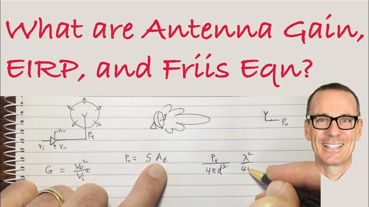
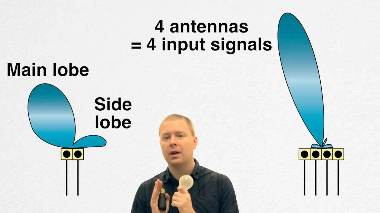


Antennas are characterized by several key parameters: solid angle (dΩ = sin(θ)dθdφ) defines the three-dimensional radiation pattern; normalized radiation intensity (F) scales the pointing vector to 100% for directional analysis; antenna patterns show radiation distribution in linear or decibel (dB) scales where dB = 10log(P/P₀); directivity (D) measures how concentrated radiation is in preferred directions (e.g., short dipole D≈1.5, 9λ dipole D≈6); radiation efficiency (η) is the ratio of radiated power to input power; gain (G) combines efficiency and directivity (G = η×D); effective area (A_e = λ²D/4π) describes reception capability; and the Friis transmission formula (P_r = P_t × G_t × G_r × (λ/4πR)²) calculates received power based on transmitted power, gains, wavelength, and distance.
Antenna Properties and Terminology Explained | EM Theory
Added:hi welcome to the next in our series of practical electromagnetics for engineers today I'm going to be very briefly going through some of the terminology we use to describe properties of antennas and you might sort of consider this a storm of terminology since things are going to be coming thick and fast and you may have to go back and watch the video several times it turns out that antennas are an old field there's a lot of terminology around um and you have to learn the vocabulary if you're following along in my class um sections 9.2 and 9.5 of the textbook are the ones you want to look at so you've seen this slide before we know that basically antennas are devices to optimize and control the emitted radiation um so that you can couple electrical engineer energy through space from one circuit to another um and what we're really going to be talking about today is the ways Engineers characterize the properties the terms they use the way they Define these things so they don't have to solve Maxwell's equations in each case um so we're going to be talking about the directional strength of the radiated field the power in the radiated field we'll talk very briefly about the real part of the resistive part of the impedance but it's beyond the scope of this class to get to the complex parts and we're going to basically be skipping these other two points down there because they go beyond where we're able to in the amount of time we have and so again the point of this is to discuss the terminology that's used to characterize antennas so before we really get into some of the detailed terms we have to understand something from geometry called a solid angle and the geometry of solids are the geometry of three-dimensional things so I think the term solid angle just means three-dimensional angles and essentially remember we have a system where we have some some source of energy with its own internal impedance we drive a transmission line and hope we've hopefully we've matched our generator to our transmission line we send a signal down and ideally the the energy we send down is going to be radiated out from this antenna structure and let's just take this antenna structure and put it in the center of a sphere and the reason we're putting it in the center of a sphere is that we assume that this radiation is going to go out into three-dimensional space maybe not in all directions but certainly we have to consider a spherical area around the sphere if we want to understand where the radiation is going and this idea of solid angle basically means that at some point far away we want to look at how much of the total emitted radiation we're capturing and so the way to think about it is we have some area that I've done in the sort of light blue color we call Delta a there so Delta a is given by this formula right here it has what you'd expect you've got an R squar term because the area of the sphere um increases as R squar so the bigger R is the bigger that area is going to be it also has two sort of angles Delta Theta and Delta V Delta V is just the angle that direction how wide that is Delta Theta is the same thing but in that vertical direction right there so this is Delta Theta and this is Delta V and it's also got somewhat of a surprising term sin Theta and this is because when the angle Theta is small it's up here near the z-axis um these sort of lines of longitude get closer and closer together the closer you get to the pole so the sin Theta term just accounts for the fact that these lines red lines here spread out as you get close to the equator so again the area is given by this formula um the solid angle is essentially just normalized to the radius we get rid of the r s term and we use D Omega for that where where this up upside down horseshoe is a capital Omega so don't get that confused with ohms it's an unfortunate um notational mix and the reason we're spending a lot of time talking about solid angle is is this notation right here um is going to appear a lot in the terminology we discussed so that when you see this sin Theta Delta Theta Delta V you know that's just sort of the an solid angle the angle at which something is admitting and that's essentially related to the amount of area we're capturing radiation from so let's just start right into our death march of terminology uh the first thing we want to know is the um Power that our short dipole that we're going to use as an example system through all of this we want to know the power it's emitting and of course we know the time average power from any radiation Source um give that creates an electric and magnetic field is given by the pointing Vector we learned before that the pointing Vector that's s is essentially just the cross product of the electric and magnetic fields and if we want to know the time average power we have to just integrate over one cycle of the wave one period in time um it turns out that if we take our farfield magnetic and electric fields from a short dipole um take the cross product of course uh F and Theta are the two directions and F cross Theta gives us the r Direction so all the the the radiation is going outward away from the center which makes a lot of sense to us um what we're going to get is we're going to get this term right here when I just plug the values in for short dipole and essentially what you see is some complicated terms We have basically the impedance of free space we have the square of the current that flows in the antenna we have the square of the length of the antenna and remember in our short dipole the length has to be much much shorter than the wavelength of light we've got the propagation vector k and remember K is equal to 2 pi over the wavelength um we've got some terms in the bottom including how far away we are and most importantly we have a s squared term and so essentially what we're going to see is the radiation from our dipole antenna the radiation power scales a s squar and we'll look into this a little bit later another term we use a lot is the total power radiated from an antenna um and this is essentially just the power that goes out in all directions the total amount of power that comes off of that antenna uh again we know our pointing Vector is power per unit area um and the unit area is given by what we just talked about this R 2 sin Theta Delta Theta Delta V that I showed you on the previous slide and so if we want to find the power radiated from say this antenna right here what we're going to do is we're just going to sum up the overall pointing Vector over all the little areas that make up the sphere and if I basically plug my equation in for um Delta a the area I come up with the second equation down here a way to intuitively think about this is if we have a little antenna again we've got this little antenna there it's a dipole uh we essentially put a sphere around the dipole and essentially what we're going to do is this integral is just going to start to take these squares and take the power through that one plus the power through that one plus the power through that one and so on and so forth all up and down the sphere that's all these integrals are doing is summing up the power through each little area where each of these little boxes is Delta a the equation looks complicated but it really isn't at all um because it's just adding up lots and lots of little boxes don't let the math scare you now Engineers don't like exact formulas we like to use sort of rules of thumbs and heris sixs um or or basically sort of catch all things and so we try to simplify our notation as much as possible so one of the things that's used a lot in antenna Theory and characterizing antennas is something called the normalized radiation intensity and I have no idea why they use the variable f for this it doesn't make sense but but it's this normalized radiation intensity is given by the variable F and it's a function of the angles Theta remember Theta goes in that direction around our sphere and F where Fe goes around in that direction and the word normalize just means that we are going to ignore the total amount of intensity and scale everything to 100% And the way we do that is we just basically calculate the pointing Vector as a function of the the three-dimensional coordinate system we're in which is the distance the angle Theta and the angle V and divided by the absolute maximum value um so we basically normalize this to one so the largest value that the normalized radiation intensity can have is equal to one and you may be thinking gosh this doesn't make a lot of sense because we've basically taken the pointing Vector which is you know hard enough to figure out and and now we've defined a new term from it and remember that the pointing Vector for the dipole is this equation right here which which is kind of a scary looking equation even though it's pretty straightforward the nice thing about the normalized radiation intensity is if you actually go ahead and do this um you plug in the pointing Vector up at the top you take the maximum value here and you'll notice that basically the maximum value of the pointing Vector is going to occur when Theta is equal 90° and so basically this just turns into one that means this term and this term cancel out and instead of having to deal with this equation calculating the normalized radiation intensity essentially just allows us to deal with the change in the intensity as a function of angle so it's really a much simpler term this is a good time to maybe explain a little bit how this works because we know that the normalized radiation intensity as a function of theta and Fe is basically equal to sin squ Theta for a short dipole so essentially how does this work our dipole is in the middle of this steroidal thing this is essentially the emission pattern as we've seen before from a dipole antenna and essentially Theta varies in that direction essentially in a plane right there so if I were to take a plane and essentially cut my plane through there this direction is the Theta Direction um the Fe direction is a horizontal plane that's the plane that cuts through the perimeter as we've seen right here in the way we've defined things and so to give you a sense of what this normalized radiation intensity looks like we draw diagrams that look like this one right here essentially the blue line is the Theta Direction so I've gone ahead and erase Theta and I'll draw Theta in so Theta is essentially in this direction right here the red line is the Fe Direction and I changeed colors again so the Fe direction is this way and so if you essentially look at the normalized radiation intensity s what you see is that s of theta that's the Blue Line essentially has the shape of this toroid it essentially gives gives us the overall radiation pattern as a function of the angle Theta um s of Fe is the red line it essentially gives us the overall radiation pattern and it's just a circle because it's the same in all directions um as you can see from that diagram right there and we'll get into this a little bit more later so if you're a little bit confused by this don't worry about it um because we're going to cover this more later the overall story is normalized radiation intensity simply uh is one in the direction that most of the radiation goes and it essentially tells you how the power of the radiation or the intensity of the radiation changes as a function of angle away from the antenna in both the Theta and the fet now these diagrams that I drew before um are known as antenna patterns and it turns out that Engineers Express these in both linear as well as logarithmic terminology um and so the graph of the normalized intensity is a function of angle is known as the antenna pattern so when you're you hear the word antenna pattern you know it's a graph that shows you the the normalized intensity as a function of the the angle away from some axis on the antenna and essentially this is going to tell you as an engineer the direction to point your antenna to get the strongest signal it turns out that for many antennas um they really emit much more strongly in particular directions by factors of a 100 or factors of a thousand because this can be really difficult ult to plot on a linear scale we often plot things on a logarithmic or decibel scale and so just to remind you here's the equation right here to convert power to decb it's essentially 10 log base 10 of your ending power divided by your starting power um and if you're working with Fields you have to square the fields and that makes the factor 20 out here um this is the scale you can use for decb it turns out that if if the ending power is is basically.1% or 1/ 1,000th of the starting power when you plug into your deciel equation you're going to find that that that power is minus 30 Deb um if you get a 10th the power it's - 10 DB um at a fifth the power it's - 7 A3 the power it's about Min -5 half power is-3 DB um it's 0 DB which is a little bit confusing if the ending power and the starting power are essentially the same if you actually get gain you get more power out you just reverse the scale twice the amount of power is plus 3 DB 3 times the amount of power is about plus 5 DB and so on and so forth lessons here negative decibels correspond to loss positive decb correspond to gain zero decb corresponds to no change this is the type of thing as an engineer you should probably memorize because you're going to see this a lot and it's good to have it at the front of your mind so let's dig into this idea of an antenna pattern a little bit more and see what some antenna patterns look like for the short dipole which is the antenna system we've learned about so we'll use to do most of the illustrations um often times on antenna pattern diagrams you essentially will see somebody draw the antenna in so I'm going to draw a little tiny line there to indicate the dipole is pointing in that direction um I'm not going to plot the change of the radiation in fee because as we go around it doesn't change in the Fe direction or essentially as a muthal direction it only changes in the the elevation direction as we get up away from the dipole which we might expect and so basically I'll put the Theta there to say this is a linear scale in terms of theta so how do we read this diagram if we're essentially normal to the axis of the dipole um so we see the currents going up and down up and down we see that the we have essentially the maximum of the radiation pattern which is equal to one here we're reading this scale is the concentric circles as we start to inrease in angle and get to an angle of about 30° either plus or minus off of the perpendicular to the dipole antenna so we're essentially maybe sitting up above our antenna at an angle of 30° there we see that we get less power we're going to get maybe something like 75 or 3/4 of the power as we go out here to maybe 45° which is midway between 30 and 60 we're down it looks like to about 30% of our power and as we start to get vertically away from our dipole more toward the axis of the dipole this number drops down to essentially zero when the current's pointing right at us it turns out the dipole radiation is symmetric across the axis but not all antennas will be some will radiate much more in One Direction in another than another as we'll see later on what's just appeared is exactly the same plot but on a log scale where we're looking at the change in the elevation or the Theta direction again if we look straight out horizontally and our dipole is going up and down in that direction right there we see a maximum value remember that that log scales are are much less sensitive to small changes um but allow us to plot big changes on a vastly expanded scale and so these two graphs the two blue lines are exactly the same but here we're plotting one which is 0 DB minus 10 DB is 1110th minus 20 DB is 1/ 100th minus 30 DB is 1 1000 and so you can see still out here when we get to 30° we're down a little bit but it doesn't really show up on the log scale when we get out here to 60 degrees um we're down considerably um in terms of decb and then so on and so forth and so essentially you can see we can represent the information either on the linear scale or the log scale depending on what information you look for that's essentially how you're going to represent the antenna pattern linear scales are good if you want to know small variations near the direction the antenna emits the most log scales are good if you really care about the small Powers there that are emitted in other directions because they allow you to see those and quantify those values better there's yet another way that we often see this done where you essentially create a three-dimensional plot in terms of theta and Fe the azimuthal and elevation directions and this is the plot for the dipole that essentially goes from 0 to 360° in the asmal plane and says that for any particular value of theta um the radiation doesn't vary in fee but as we go from theta equals 0° to 90° which is normal to the dipole and then back down to 180° which is pointing at the dipole from the bottom what you're going to see is that this type of radiation pattern and so you'll sometimes see radiation patterns or antenna patterns shown in these types of three-dimensional diagrams as well if you really want to capture information about both Theta and Fe in one graph remember in these this graph here and this graph over here we're only looking at the Theta variation not the fee variant well Engineers often want to talk about um how good an antenna is about sending radiation a particular direction without having to look at a graph and in this case we use a number called the directivity and we use the variable D for that and directivity of an antenna is simply a single number that tells you how much the antenna wants to radiate in its preferred Direction the direction where the radiation is the strongest and it turns out that antennas with low directivity and uh directivity D equal 1 is the lowest possible radiates equally in all directions so if you're given antenna with a d of say like 1.1 you know pretty much any direction you're going to get a signal from antennas with very large directivities tend to create one or more narrow be mes of radiation um so if you don't know the direction the odds that you're going to pick up a signal are pretty low with a high directivity antenna you essentially calculate the directivity by calculating the max of the normalized intensity or normalized radiation intensity and divide the maximum value by the mean value and the mean value of course you just have to integrate um over your sphere again remember this this means we're integrating over a sphere um another way to to put this is the maximum value of the pointing Vector S as a function of r Theta and V / 4 Pi r^ 2 divided by the total radiated power that total radiated power will get to in a little bit but it's just the power that's radiated over all directions so so let's clarify this directivity D by looking at some examples of a small dipole but also some longer dipoles as we'll talk about in the next mini lecture here we have the radiation pattern of a short dipole um basically we know that it's um normalized radiation intensity is normal to the direction of the dipole if the dipole is going that way and it's equal to one out here um it doesn't really want to radiate in a preferential Direction the directivity is pretty low it has a value of 1.5 um for the short dipole where the length of the dipole is much much less than a wavelength if we go ahead and plot the radiation pattern for a longer dipole this one's three wavelengths and length and I'm basically getting these graphs from this website down here that you can all go to and plug in the numbers and generate these curves yourself um this has a directivity of three and if we look at the radiation pattern and compare the two you'll essentially see that this is a much more directional radiation pattern there are some directions it really wants to radiate in but if you're sitting at at this angle you're not going to see anything and as the dipole gets longer here we're looking at a dipole that's nine wavelengths in length um it becomes much more directional you get sort of narrow loes and it's only going out in particular directions um and this has a directivity of about six um for the longer dipole and so you really see that the number of directivity doesn't tell you at all the direction the radiations going but it does say you have a more narrow beam from that end on to the next um animal in our zoo of terminology this one is called the radiation efficiency it's given by the Greek letter Z and the rad radiation efficiency is just the ratio of the total power that's radiated from the antenna in all directions to the total power you drive it with so again we think of some sort of generator driving a transmission line that's matched and then the transmission line sends a signal down to the antenna um some of the antenna or some of the energy that goes or power that goes to this antenna is going to get radiated off as a wave we can detect um Others May other power May simply heat up the antennas or be lost due to resistances within the antenna and so essentially what the radiation efficiency tells you is how much power that drives the antenna actually goes out into free space and of course we need to calculate the radiated Power by basically putting a sphere around our antenna and doing the integral summing up all these little squares as we've seen before earlier in the video this involves a double integral but it's not that hard to do so a good way to think about the radiation efficiency is how good the antenna is at converting the power you give it into some kind of signal that will propagate through space that you can detect later on another term that's related very closely to the radiation efficiency is something called the gain g and the gain is really pretty simple it's just the radiation efficiency Z multiplied by the directivity D again radiation efficiency multiplied by directivity um so you can see that even if the radiation efficiency of an anten is pretty low it loses some energy to heat it doesn't all go into space if the directivity is high the gain can be greater than one so the power in a particular direction um can be more than the power you drive the antenna with if the antenna is directional and the directivity is G greater than the gain and this is a little counterintuitive because how can we get more signal than we put in the answer is we don't we only have more signal going in one particular direction than we would if we radiated in all directions and so the key point an antenna can have significant losses and still have gain if it's highly directional even if the radiation efficiency is not optimal so let's dive into this concept of efficiency in a little bit more detail by defining another term um of the antenna something we're actually familiar with we've learned before called radiation resistance again we have our system where we have some generator sending a wave down our transmission line driving our little an one way to think about this system is essentially a current Source that's going to drive the currents remember currents are what radiates an antenna current that's going to drive the currents in this antenna and we can make a schematic model a circuit model of our antenna um in a very simple case ignoring any impedances which we're totally going to skip over um as we talk about this stuff even though they exist and think about the resistance of of the antenna and really there are two series resistances to this antenna the loss um that's due to Heating and due to the resistance of the wires the antenna is made out of and some antennas are pretty big and there's a long length of wire so this can be pretty significant as well as a thing that's not really a resistance but is power lost to the radiation that basically comes off the antenna and hopefully goes in the direction you want it to so it can be detected um we use ohms law and basically can talk about the power that goes to loss which is basically 1/2 the driving current squared times the loss resistance and a similar term for the radiated power being equal to the power calculated from ohms law well we already know about this loss term we can calculate the loss resistance pretty easily so let's pop in an old slide um where we see the loss comes from the surface resistance remember we've calculated before how the resistance of a wire is actually a function of frequency because its frequency gets High um all all of the current flows in a thin region around the circumference of the wire and we essentially by knowing the conductivity Sigma and the the loss as a function of depth in The Wire Alpha we basically can calculate the loss resistance using that equation right there which is dependent on the square root of the frequency and we saw in a previous example that at DC you can have low resistance but the resistance becomes pretty significant when you Jack the frequency up to 1 GHz so basically that's how you take care of the Lost term right there the radiation resistance is a little bit tougher essentially you have to calculate the total power radiated um again we basically just take the pointing vector and we integrate it over the surface of a sphere I told you you'd see these integrals a lot as we went through this lecture so that's one way you can calculate the radiated power um other ways you can calculate the radiated power through the directivity because the direct ity is the maximum pointing Vector divided by the total power radiated into a sphere that's going to basically be the average power which is our definition of directivity so if you know the directivity of an antenna D and you know the maximum pointing Vector there is a shortcut to calculate the radiated power P radiated well once you get the radiated power um from the directivity or or directly by doing this integral then basically we just use a little bit of algebra to convert the radiated power over to the radiation resistance which is given by this term right here and if you go ahead and plug everything in and do the algebra you're going to find out that the radiation resistance of a short dipole is uh given by this equation right here and so let's stop and take a look at these numbers you know 80 pi^ 2ar is something like 80 * let's call it roughly 10 so this first term is going to be about 800 but we also know in a short dipole that the the length is only a very small fraction of a wavelength typically D is less than a 50th of a wavelength so essentially this number is going to be something like 1 over 50 and if you square that you get 1 over 2500 so the radiation resistance is going to be a fraction of an OHM for a short dipole antenna for bigger antennas the radiation resistance becomes significant what does this tell you um it's not easy to drive a very short dipole antenna so let's take a look at why that is again we think about our our our system where we have some generator driving a transmission line that took to our antenna and this antenna is a short dipole D much much less than the wavelength of the radiation the wavelength on the transmission line um we can think about this system essentially as just a transmission line if we have an an equation Z no and so we're driving Z antenna um and we know the overall impedance of the antenna is the loss resistance plus the radiation resistance and we know this is basically pretty much less than one plus whatever kind of um reactive or imaginary component we have what this says is it's probably the imaginary component that's going to dominate the term and so that while the load impedance is going to be complex it's going to be more imaginary and the reflection coefficient is high so one of the problems with short antennas is they don't radiate very well and because they don't radiate very well it's hard to drive them with with a reasonable Circle okay that pretty much covers all the basic terminology we need but we need to consider something else um which is that we don't only want to take signals and send them into space uh we want to be able to receive those re those signals once we put them out into space or they don't do us any good um and so now we bring in an idea called reciprocity and this is really important and it's a basic concept essentially what it means is that an antenna that is effective at transmitting can be used to receive and so if we take some antenna here and it's essentially sends out a signal in this direction and take an identical antenna and put it over here that this second antenna is going to be a good receiver at least as good a receiver as the transmitter is a good transmitter and so we don't have to design separate antennas for transmitting and receiving they work for both which is actually really convenient and it actually turns out to be easier than you might think to calculate the receive signal um if we're far away and let's go out in the far field so we don't have to worry about weird terms in the electric field uh we can think of this transmitting antenna essentially as putting out waves and out here over at the receiving antenna far away these are pretty much plain waves um so essentially we're going to have a pretty flat phase front um pretty constant electric field distribution coming into this antenna and so how do we think about a receiver antenna work now now this is not a good technical analogy but if I think about my transmitting receiver here so let's write transmit over here and basically receiver over here um if I think about my transmitting antenna sending out a signal this way toward my receiving antenna I like to think of the receiving antenna not as an antenna but as a net and we've got these plane waves that are coming in here and we simply need to know how much of the power contained in this plane wave we're going to capture well we know this is a pointing Vector s which is essentially the watts per square meter or watts per unit area so one way to calculate how much power we're going to capture is just to calculate the area of the net that the antenna will pick up and so one can think about let's erase all that chicken scratch well one can think about essentially the antenna effective area as being equivalent to essentially a net and it turns out to be fairly easy to calculate on on effect area for an antenna and that's basically just the power intercepted divided by the power incident and that turns out to be um the wavelength of the radiation squared multiplied by the directivity divided 4 pi and as you can see um this number because D is unitless is in in in terms of meter squared or in area so if you know the directivity of an antenna you know at least if you point it in the right direction it has an effective area given by this term right here so think about antennas is catching some of the field that comes along in their vicinity now once we capture that that um once we capture that signal we have to get it to some kind of receiver so I've drawn two systems here this is our transmitter so let's write transmit up here we have a generator driving essentially a transmission line it drives an impedance this edance is an antenna it emits radiation which goes out in some direction hopefully the direction we want and hits an antenna which captures like in that some of this antenna the signal goes back into some kind of receiver circuit that has a an impedance and we're going to ignore the effect of the transmission line and just think about the receiver and the antenna impedance to keep things simple you guys know how to match transmission lines if push comes to shove well if we think about our receiving circuit over here and so let's write receiver down there um we've got two impedances we've got the impedance of the antenna um which has basically a radiation resistance plus some uh reactant some imaginary component an inductance or capacitance that we're not going to talk about and the receiver over here also has an impedance which is the resistance of the receiver plus the reactants and I should probably put a j out there um just to be consistent and it turns out that you get the greatest signal on your receiver when you match the impedances and this maximum power trans transfer from the receiver or excuse me from the antenna that's capturing the signal into the receiver occurs when the resistances are equal and the reactances are negative of each other or to put more simply in engineering terms the antenna impedance is the complex conjugate of the receiver impedance this gives you the maximum power um transfer and helps you design antenna impedances and also pick receiver impedances to detect small signal okay we're almost done with our ter ology we're on the last equation so stick with me here um we're essentially going to talk about a transmission formula that essentially tells you the ratio of the received power to the transmitted power so how much power you receive on your detector or receiver assuming it's well matched compared to the amount of power total amount of power you transmit and essentially um this is calculated by basically taking the effective area of the receiver um multiplying it by the efficiency of the receiver multiplying by the area times the efficiency of the transmitter this essentially just gives you an amount of of power and then you need to divide this by the wavelength squared because it turns out that the um sizes are given in terms of wavelength that's what counts that's why that Lambda appears there and also divide by the distance because of course this power is going to go out and scale as the square of the distance because we're assuming it has some sort of spherical dependence in the area of a sphere depends on its radius um this is one way to calculate it it's easier to think if you know the gains of the receiver and the gains of the transmitter this is something that's maybe given to you in a data sheet um that the overall um ratio between the receiver power and the transmitter power is given by the the product of the gain of the receiver times the gain of the transmitter multiplied by that factor right there which is given by um Lambda over R SAR with a 4 Pi Factor again as you get further and further away the overall received power is going to drop off as a square of the distance um and then you multi you basically adjust that with the gain terms it's it's a complicated formula but it's actually fairly straightforward and makes a lot of sense intuitively if you just think about the power dropping as Lambda over r squared and what I've given you down here is so you don't have to go back in the video the formulas for the effective areas in terms of wavelength and directivity the gain in terms of the efficiency in the directivity the um efficiency in terms of radiated and total power and our expression for the dir activity here what you're seeing with all these formulas is there's um a lot of remembering what's what and a lot of algebra involved um but Engineers essentially have manipulated this so they have numbers to work with so they don't have to do a lot of integrals for every problem of course this transmission formula only holds if the the antennas are oriented so that the um gains are maximized they're pointing in the right orientation to each other if you essentially do what I've shown in the figure that just appeared and you sort of tilt these antennas so they're not in the direction you basically um have this antenna tilted so it's not in the direction that has the maximum gain and this one in not in the direction that has the maximum gain essentially you take this this previous equation and multiply it by the normalized intensity as a function of theta and Fe where Theta and Fe for oops let's get these right and multiply it by the normalized intensity is a function of theta and Fe where essentially the normalized intensity for the transmitter tilt is over here and the normalized intensity for the receiver tilt is over there this is just an adjustment Factor if your antennas aren't oriented that's everything we done um you'll probably have to watch this several times to get all these terminologies but this will at least give you the vocabulary you need to read about antennas and understand some of the terminology that Engineers use to describe various antenna types
Up Next

Electromagnetic Waves & Maxwell's Equations: Physics Lecture
@Cornell
556.9K views•2009-07-30

21cm Hyperfine Transition in Neutral Hydrogen: Radio Astronomy Basics
@AaronRobertParsons
12.4K views•2011-10-13

Gaussian Beam Propagation: Parameters and Calculations Explained
@kridnix
65.3K views•2009-01-30

Entropy and the Second Law of Thermodynamics Explained
@veritasium
27.5M views•2023-07-01
Related Study Plans & Knowledge Roadmaps
Structured learning paths in Physics