Robotic Inverse Kinematics Algorithm for Hexapod Leg Design and Control

[00:00:00]So I want to make a hexapod, a cheap hexapod,  they look interesting and are a great start but for something that walks, because they  are stable. I'm going to split this into multiple videos because there's just so much  to cover, in this one I'll talk about inverse kinematics and how to make a hexapod leg  walk, in the next video I'm going to make the whole hexapod and hopefully have it  walking and running all over the place, and in the final video I'm going  to make the hexapod remote control.

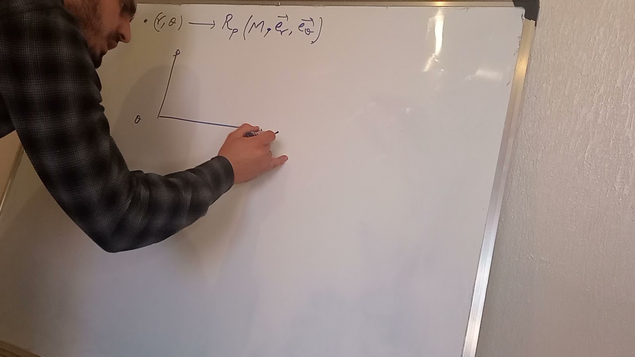
[00:00:30]Welcome to Just Another Maker Channel. So how  do we make a hexapod walk? It all comes down to inverse kinematics, what is inverse kinematics?  Well kinematics is about the motion of objects, so the kinematic part is we want  to move this, from here, to here.

[00:00:51]The inverse in this sense is the  'how' do we get from here, to here.

[00:00:57]I'm going to go through the inverse  kinematic solution and then I'll demonstrate it working along with  some of the mistakes I found while doing this and give a quick overview  of the programming code at the end.

[00:01:13]Now if we take the hexapod we are hopefully going  to make, and first we say this is the front, this is the leg we're going to focus on for our inverse  kinematic solution. We define our coordinate system, so this is our x-axis, this is our y-axis,  and this is our z-axis. I know this might seem a little bit strange but this coordinate system  is used commonly with industrial robots.

[00:01:39]Ultimately the letters X Y and Z don't matter,  they could be called A B C or Rock Paper Scissors, but we'll stick to XYZ. It can also be  easily remembered using a right hand like so, with the fingers pointing  in the positive direction.

[00:01:56]So if we put this to one side and  look at our hexapod leg from the side, it's controlled by three micro servos, we  will label these as joint 1 J1, J2 and J3.

[00:02:11]To try and make it as clear as possible here is  our hexapod leg from the side and from above.

[00:02:16]Here is our coordinate system, J1 is underneath  here and rotates like this around the Z-axis, J2 rotates like this around the X-axis, and J3  rotates like this in essentially free space; but we'll get to that in a minute. First  we're going to solve a 2d inverse kinematic solution for J2 and J3 with our leg  in the rest position as it is shown, ultimately we are trying to control where the  foot of the leg is placed; this point here, now we can draw a triangle through the centre of  J2, J3 and the point we want the foot to be at.

[00:02:54]We need to know the angle for J2 relative to  the Y-axis and the angle of J3 relative to J2, we know the length of the J2 segment is  57mm in this case, which we will call J2L and the length of the J3 segment  is 110mm which we will call J3L, we need to calculate the length of the  remaining side; for now we will call this L.

[00:03:19]We can calculate L using the following  triangle and Pythagoras Theorem, we already know the other sizes of this  triangle because it's where we want to position our foot in Y and Z, and we  know that Y is at right angles to Z.

[00:03:35]Pythagoras Theorem tells us that the square  of the hypotenuse, L in this case is equal to the sum of the square of the other two  sides here that is Y squared plus Z squared, so the length L is equal to the square root  of Y squared plus Z squared. Now we can solve for the angle J3 using the law of cosines the  law of cosines tells us that to find the angle D for a triangle where we know the lengths of all  three sides that D equals the inverse cosine of A squared plus B squared minus C squared, divided  by, 2 multiplied by A multiplied by B. So to solve for J3 we can just substitute our values  which gives us: J3 equals the inverse cosine of J2L squared plus J3L squared minus L squared  divided by 2 multiplied by J2L multiplied by J3L.

[00:04:39]All that remains is to find J2. for this we need  to find two more angles which we will call A and B to find angle B we can just  use the law of cosines again, and just substitute our  values in which gives us this.

[00:04:57]Angle A is also present here in this triangle,  to find angle A we need to use some simple trigonometry; there are three trigonometric ratios  for right angle triangles and in this example we need to use the tangent of angle A equals the  opposite side Z divided by the adjacent Side Y.

[00:05:16]However we want to find the angle,  so we can rearrange this to: angle A equals the inverse tangent of the  opposite side Z divided by the adjacent Side Y.

[00:05:29]And finally to solve for J2 it's  simply angle B minus angle A, and that's all there is to it! Now to  3D print some parts and assemble them.

[00:06:12][Music] I've designed the 3D printed parts so  that I can glue the servo horns into them.

[00:06:18]One of the key things to assembling this, is to  make sure the servos are at a known position, here I am turning the servos back and forward to  try and find the centre point of their movement.

[00:06:39]I use a two-part glue, it's actually mitre  adhesive; it's a CA glue and spray activator that makes it set quickly. It seems to work  quite well with the 3D printed PET. To secure the servos I'm just using the self-tapping screws  that came with them. The 3D printed parts do have some 1mm holes printed into them, though they  seem to have closed up slightly during printing.

[00:07:08]This servo doesn't seem to want to turn,  unfortunately it's broken fresh out of the box.

[00:07:42]Now everything moves nice and smoothly, I'm just going to tie these cables up nicely  out of the way and we can get testing.

[00:08:00]So here I have the J2 and J3  servos wired up to an Arduino Nano, let's download some code that uses our inverse  kinematic solution and see what happens, the leg should start at the rest  position and move 100mm in Y.

[00:08:29]Well that didn't quite go as planned, so what  went wrong? Multiple things went wrong all at once, and they are related to how it is  assembled and how the servos are controlled.

[00:08:39]Firstly because we're using servos, the  range of motion is zero to 180 degrees, so zero degrees for J2 in our kinematic solution  is directly along the Y-axis; but for our servo that is 90 degrees. So to get the required servo  angle, it is equal to 90 minus our calculated J2 angle. The next issue is that, if I'm asking  this to move to Y equals 40 and Z equals 0, which in our solution is roughly here, but in  reality I want this to be relative to the foot, assuming this point is our rest position, so  all we need to do is apply some offsets. Say it 90mm in Y and minus 60mm in Z. so when I say a  go to Y equals 40 and Z equals 0; what we really do is calculate the solution for here, Y equals  90 plus 40, which is 130 and Z equals minus 60.

[00:09:36]The other key element with J2 is angle A,  because our resting Z offset is negative, angle A is negative; J2 equals B minus A,  so B minus A ends up being B plus A, because two negatives become a positive. So we need to  invert the minus in our solution to a positive.

[00:10:00]J3 is a completely different kettle of fish.

[00:10:05]We calculated the angle of J3 relative to J2 but  our servo was not mounted in line with our foot, so we need to measure this angle from our  design and added onto our J3 solution.

[00:10:18]Now in order to maximize the  range of motion available; I fitted the servo horn here when the  servo was at 90 degrees. This means we need to subtract 90 degrees from whatever we  calculated to find the correct servo position.

[00:10:32]So we can see that with the changes  we can request 40mm movement in Y.

[00:10:43]And also 40mm movement in Z. Now  that we have Y and Z working with J2 and J3 we can look at X and  J1; this is actually quite simple.

[00:10:57]If we take a look at our hexapod leg  from the top, it looks like this, and it operates within the X and Y  coordinates. If we assume we want to move the foot to this point here,  then we simply need to find this angle, which as we've seen earlier can be done using  trigonometric ratios for right angle triangles; angle J1 equals the inverse tangent of the  opposite side X divided by the adjacent side Y.

[00:11:24]But by adding J1 into our solution we need to  adjust the solution for J2 and J3, because they no longer operate within the Y and Z axis, but  operate along this line here; which we'll call H.

[00:11:37]We can calculate H using Pythagoras  again; which gives us this.

[00:11:41]So now we just go back to our J2 and J3 [Rewind  Effect] and we can swap Y for H here, here, here and here. And that's it! Our inverse kinematic  solution is finished and it looks like this... 40mm forward in X You might have noticed that while we end up in  the right places, our leg doesn't get there in a straight line. The reason is because our  servos all need to move different angles, and by only commanding them to go to the end  position, they all start at the same time, and some of them get there first because  they don't have as far to travel.

[00:12:40]So to fix that we need to use interpolation.

[00:12:44]Instead of commanding our servers to move all the  way to the end in one go, we split this up into separate moves, and each move it will still hop,  but the more moves we split it up into the smaller the hops, and we can achieve a straight line. So  now we can make it go where we want, how we want, we can make it do this... Here is an example  of it drawing straight lines with 10mm spacing, unfortunately there are a number of factors  that make the lines not truly straight, like the dead band of the servos, the inertia of the arm,  friction between the pen and the paper, and just the general cheapness of the servos. Nonetheless  I still think this is pretty impressive.

[00:13:25]Here is a short walking animation that  I plan to use for the finished hexapod.

[00:13:30]In theory the legs will move in two  groups of three for normal walking, so I'll need to transpose these values to suit  the legs that aren't perpendicular to the body of the hexapod, but that's for another video! The  code for this is all quite straightforward, all of the hard parts have been covered earlier in this  video, but it essentially comes down to these nine lines of maths. There is a link in the description  so you can download the chode yourself and use it or adapt it for any of your projects. I hope you  found this video interesting and informative. In the next video I'm going to stick six of these  onto a base and get a hexapod running around.

[00:14:18]Thanks for watching guys don't forget to Like,  Comment and Subscribe! See you in the next one!