


















![STUD[IE] UTS PE-2 21/22](https://i.ytimg.com/vi/xlWJkiq2E1Q/maxresdefault.jpg)
![[풀버전] 미국의 '부채폭탄, 국채시장 흔들릴까? 달러 스테이블코인이 가져올 '과잉 유동성'은 버블붕괴로 이어질 것인가? | 클로즈업 - '위험한 유동성'](https://i.ytimg.com/vi/1F9g25R0Uyw/maxresdefault.jpg)





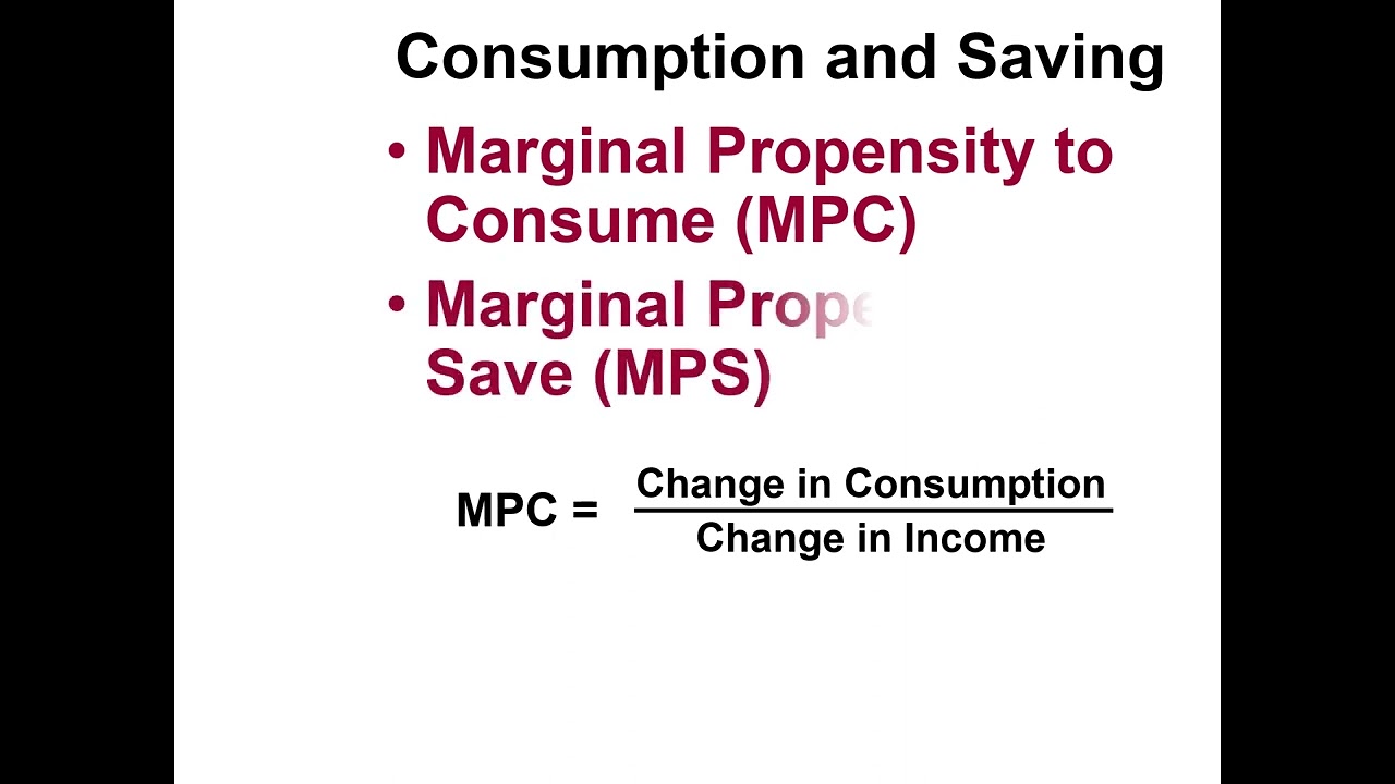
The government spending multiplier measures how much aggregate demand increases from an initial increase in government spending, calculated as 1 divided by (1 minus the marginal propensity to consume); a higher marginal propensity to consume results in a larger multiplier effect, meaning less government spending is needed to close a recessionary gap, while a lower MPC produces a smaller multiplier requiring more spending to achieve the same aggregate demand increase.
Fiscal Policy: Government Spending Multiplier Explained (Economics) | AP/IB Macro
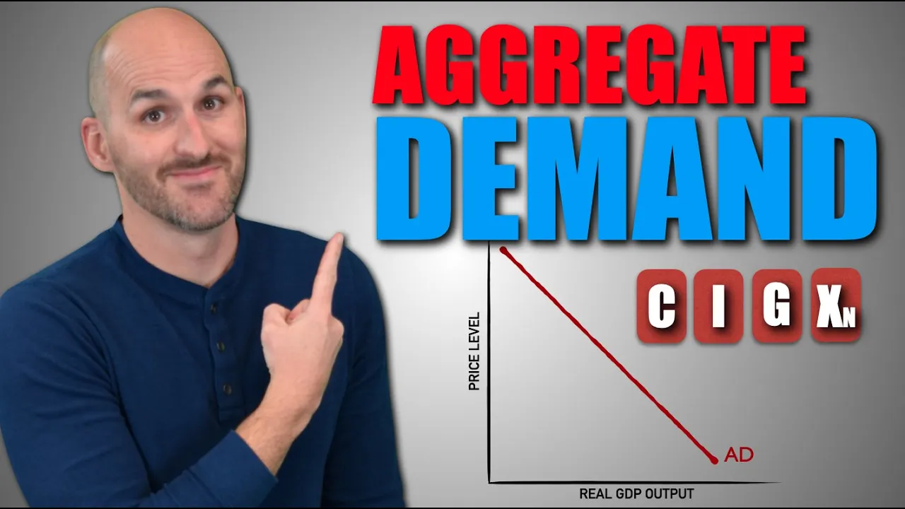
Added:Understanding the components of Aggregate Demand (AD = C + I + G + NX) and how shifts in these components affect the macroeconomic equilibrium.
The basic definition of Fiscal Policy, specifically distinguishing between expansionary and contractionary government actions.
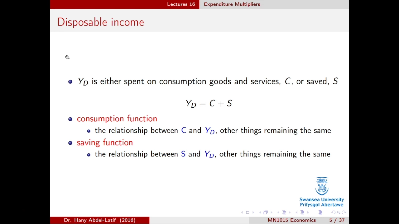
The concept of disposable income and the fundamental economic behavior of households dividing income between consumption (C) and saving (S).
Familiarity with the Circular Flow of Income model, showing how money moves through an economy between households and firms.
The Tax Multiplier, including how to calculate it and why it is smaller than the government spending multiplier.
The Balanced Budget Multiplier, which analyzes the net effect of equal increases in both government spending and taxes.
The Crowding-Out Effect, illustrating how government borrowing to fund spending can raise interest rates and decrease private investment.
Real-world limitations of fiscal policy multipliers, such as implementation time lags, inflation pressures, and import leakages.
73.7K views411likes20:06Original Release: 2011-11-28
here we [Music] go today's video Lesson will explore the effectiveness of the use of fiscal policy by examining what are called the multiplier effects of government spending and Taxation let's begin by reviewing the definition of fiscal policy fiscal policy is when a government changes either the level of Taxation and or the level of government spending in order to promote the achievement of a macroeconomic objective of course the macroeconomic objectives a government may wish to promote are full employment price level stability and economic growth what we're going to consider today is the effectiveness of government spending as a tool of fiscal policy and therefore as a way to e either increase or decrease aggregate demand let's start by looking at a nation's economy such as that which we see on the right here here we can see that the equilibrium level of national output at present of y1 is lower than the Full Employment level of output this economy is experiencing a recessionary gap just for the sake of an example let's say that this economy's recessionary Gap or the difference between its equilibrium output and its full employment output is equal to $5 billion if this economy were producing out its full employment level its GDP would be $5 billion more than it is at present in addition to a weak level of aggregate demand this economy has a relatively low price level which indicates that there may be deflation or disinflation in the economy now a government wishes to stimulate aggregate demand and move it back to the Full Employment level it can do this in one of two ways as we learned in our previous video Lesson expansionary fiscal policy which would increase aggregate demand consists of either increasing government spending we'll call that g increase or decreasing the level of taxes now this has all been explained in a previous lesson what we will do today is evaluate the effectiveness of increasing government spending by examining what is called the multiplier effect the multiplier effect is defined as follows if a particular increase in government spending leads to a greater increase in aggregate demand than the change in government spending itself then we say that that government spending has been multiplied and will have a greater expansionary effect on aggregate demand than the initial change in spending would indicate let's just do a quick example of when the multiplier effect might exist so for example if government spending increases by $1 billion and total aggregate demand increases by $4 billion the only way this outcome could be possible an increase in ad that exceeds the increase in G is if there is a multiplier going on in the economy in other words in this case the 1 billion increase in government spending was multiplied four times result resulting in an increase in aggregate demand equal to $4 billion so this would indicate a multiplier of four how do we determine what the size of the spending multiplier in an economy is in order to do this in order to determine just how much a particular increase in government spending will lead to an increase in aggregate demand we must consider some macroeconomic variables known as the marginal propensities to consume and save next we're going to Define these terms and then decide how we can use them to find the size of a government spending multiplier before we can determine just how large a government spending multiplier will be we must know how much a change in income among a nation's households will contribute to the level of consumption in the economy and how much of it will go towards savings this is what the marginal propensities to consume and save can help us do so the first Factor we'll consider is the marginal propensity to consume which we abbreviate as MPC a nation's marginal propensity to consume refers to the proportion of any change in income among households in that nation that is used to consume domestically produced goods and services therefore the simple formula we will use for the MPC is the change in consumption divided by the change in income Let's do an example to illustrate what this really shows us let's assume that government spending in an economy increases by $1 billion and as a result the income among the nation's households Rises by $1 billion now why does an increase in government spending lead to an increase in income of the same amount this is fairly straightforward a government spends money on things that are ultimately by the households of that Nation let's say a government orders some new weapons or some new fighter jets and those fighter jets are produced domestically if the government spends a billion dollars on new fighter jets contractors the military contractors that build the Jets will hire more people or will pay the existing workers that they employ higher salaries in order to produce these new Jets to meet the government's order this $1 billion will ultimately end up in the pockets of the employees and the shareholders of the companies that make the Jets therefore income among the nation's households Will Rise by the billion dollars now what happens to the billion dollars once it is in the pockets of the nation's households of course some of it will be used to consume domestically produced goods and services let's assume that the 1 billion doll increase in income leads to an increase in consumption of domestic output by $400 million with this information we can actually calculate the marginal propensity to consume among this nation's households a $400 million increase in consumption resulted from a 1 billion which is equal to $1,000 million increase in incomes this gives us a marginal propensity to consume of 400 divided by 1,000 which is 0.4 with that number 0.4 what we know is that for every $1 increase in income among the nation's households consumption will increase by a further 40 cents using this marginal propensity to consume we'll be able to determine just how much the government spending multiplier will be and therefore how much additional output will result from a particular change in government spending now let's look at the marginal propensity to save which we use MPS for the abbreviation the marginal propensity to save tells us basically the opposite of the marginal propensity to consume if the households of a Nation are not consuming with additional income that they earn they must be saving with it this is a bit of an oversimplification because of course there are certain things that households do besides consume and save such as buy imports or pay taxes but for our case we're going to consider all money that is not spent on domestically produced Goods as going towards savings so the marginal propensity to save is the change in savings resulting from a particular change in income now let's use the same increase in government spend in of $1 billion and see how this might affect the savings among the nation's households assuming a marginality to consume of 0.4 so this government spending will increase household income by $1 billion which as we saw above led to an increase in consumption of $400 million therefore we assume that savings is increasing by the rest of the1 billion increase in income which in this case would be $600 million now what what is the marginal propensity to save assuming that a$1 billion increase in household income leads to $600 million of new savings the marginal preny to save is simply 600 million divided 1,000 million which is 06 now what does this tell us this tells us that for every $1 that households in household incomes rise in this country savings will increase by 60 Cs and in the case of a $1 billion increase in government spending leading to to a$1 billion increase in incomes savings increased by $600 million what we should notice right away is that no matter what the MPC and MPS are in a nation the two will sum up to or will equal one of course we're simplifying things by here by saying that households either spend or save any change in their incomes now if you're an IB economics student you must must also consider two other leakages that may occur following a change in income in IB economics we understand that savings is not the only thing households do with disposable income and in fact what may also happen is is that they may buy imports so we will also consider the marginal propensity to import which is mpm and we may also be asked to consider the amount of an increase in income that goes towards taxes which gives us the marginal rate of tax ation the MPS plus mpm the marginal propensity to import plus the marginal rate of Taxation equals what we call the marginal rate of leakage or the mrl the marginal rate of leakage refers to the proportion of any change in income that goes towards the purchase of imports savings or taxes paid to the government all three of these Imports SA savings and taxes are considered leakages what can an understanding of a nation's marginal propensity to consume and save tell us about the effectiveness of a particular increase or decrease in government spending the next thing we're going to do is determine how we can actually find the multiplier for government spending using this MPC and MPS data once we know the marginal propensity to consume and save of a Nation we can find very easily the size of the kyian government spending multiplier which we will use K as the abbreviation for now of course this is called Keynesian after the economist John mayard canes whose theories about fiscal policy form our modern day understanding of how it works so what is the multiplier the Keynesian multiplier will always be 1 / 1 minus the marginal propensity to consume now this seems a little bit complicated but it's actually quite easy to understand the implication here is that the higher the MPC in a nation the greater the multiplier will be Let's do an example here let's assume that the MPC in ation equals 0.4 what will the spending multiplier be for a nation whose marginal prty consume is 0.4 it will be 1 over 1us 0.4 which is 1 / 0.6 which is 1.6 7 what does this number 1.67 tell tell us what it tells us is that any increase in government spending will ultimately result in an increase in aggregate demand of 1.67 times that increase in government spending for example let's assume that the government spending increases by $1 billion again this will lead to an increase in aggregate demand of the multiplier times the change in government spending in other words ad will increase by 1.67 times the $1 billion increase in government spending which is $1.67 billion How would this look on a graph let's look at our graph on the right here to illustrate the effects of this $1 billion increase in government spending multiplied by the 1.67 multiplier if government spending Rises by $1 billion there will be an initial increase in aggregate demand of a relatively small amount just $1 billion so as we see here ad will shift out but the magnitude of that shift will be relatively small only $1 billion graphically we can see that when there's a recessionary gap of $5 billion this $1 billion increase in government spending Al loone will have very little effect at moving the economy back towards its full employment however once it has been multiplied due to the increasing incomes of households in the nation which leads to further increases in consumption and aggregate demand we have an ultimate increase in aggregate demand that will exceed the original or the initial increase in aggregate demand so ad will shift out by more than it does following the increase in government spending now that's a bit too much because in fact the increase in ad that will result will be just 1.67 times the increase in government spending so we'll have a new ad curve that's even further out than the original ad curve so now we see that rather than increasing aggregate demand by just $1 billion this expansionary fiscal policy increases aggregate demand by 1.67 billion now this is clearly not enough to fill a recessionary gap of $5 billion so if this government wish to determine just how much government spending was needed in order to fill this $5 billion recessionary Gap it could find this amount by using its multiplier and determining just how much G would have to increase by so to do this the Govern would want to consider two factors a what is the desired change in aggregate demand and in this case we know that is $5 billion an increase in ad of $5 billion will fill this recessionary Gap and move the economy back to its full employment level secondly the government would want to know what is the multiplier and as we saw before the multiplier was 1 over 1 - 0.4 which equal 1.67 now knowing this information the government knows that it does not have to increase government spending by the full $5 billion to achieve this increase in output rather the government spending that must be changed is equal to the desired change in GDP or agregate demand divided by the multiplier which gives us an increase in government spending of $3 billion now if the government increases spending by $3 billion so let's see government spending increases by 3 billion this will lead to an increase in ad of 1.67 * 3 which is $5 billion so looking at our graph again what would a $3 billion increase in government spending ultimately caused to happen in this economy of course 3 billion is much greater than the original change of just 1 billion so when we change government spending by 3 billion ad will shift out further to the right than it did in our 1 billion in increase in government spending but because of the multiplier effect there will be an ultimate increase in aggregate demand that exceeds that achieved by the $3 billion increase in government spending in fact it will be 1.67 times greater so due to the fact that the government understands the size of the spending multiplier this government was able to determine an appropriately sized fiscal stimulus which would shift ad out but ultimately by more than the $3 billion increase in government spending so what does this tell us about the importance of the marginal propensity to consume in a nation if the marginal propensity to consume were greater would a larger or smaller change in government spending be needed in order to achieve this $5 billion increase in aggregate demand Let's do an example here let's say the MPC equals not 0.4 but rather 0.8 let's say that for every $1 increase in income households consume 80 cents worth of it and Save only 20 cents now we would have a spending multiplier of 1 over 1 - 0.8 which is 1 over 0.2 which is five in order to achieve a change in aggregate demand of 5 billion we would only need to increase government spending Now by 1 billion so the change in aggregate demand of 5 billion divided by the spending multiplier of five gives us a change in in government spending of only $1 billion now what we see is that due to the higher marginal propensity to consume a much smaller fiscal stimulus is needed and only $1 billion of new government spending could lead to a change in aggregate demand of 5times the 1 billion which gives us a $5 billion increase in aggregate demand so in this way we've seen that the higher the marginal propensity to consume in a nation the larger the spending multiplier and the smaller the marginal propensity to consume in a the smaller the spending multiplier so to summarize the government spending multiplier tells us some very important things about the effectiveness of fiscal policy first of all the higher the marginal in marginal propensity to consume in a nation the larger the multiplier effect of government spending the reason for this is that when in when households consume a greater proportion of any change in disposable income a government spending policy that increases households income will lead to further increases in consumption in private spending that multiply or magnify the ultimate increase in aggregate demand on the flip side though the lower the MPC in a nation the smaller the multiplier effect of government spending so the the the reason for that of course is that if households tend to save more of any change in disposable income it will be leaked from the economy and an increase in income resulting from an expansionary fiscal policy will have relatively small effect on the overall overall level of aggregate demand now to conclude we could also say that the higher the MPS in a nation the smaller the multiplier and the smaller the MPS or the lower the MPS the higher the multiplier in fact the government spending multiplier can actually be expressed in terms of the marginal propensity to save as well we can also say that k equals 1 over the MPS or for IB students one over the marginal rate of leakage since in IB economics we acknowledge that in addition to savings there are other forms of leakages from a nation's economy including the marginal propensity to import the marginal rate of Taxation and the marginal propensity to save so there you have it this is the conclusion of our lesson on the government spending multiplier which is determined by comparing the marginal propensities to consume and the marginal propensities to save among a nation's household in our next lesson we're going to talk about what is called the tax multiplier you may have noticed that today we only talked about the effect of government spending on aggregate demand what happens if a government chooses to cut taxes rather than increase its spending Taxation and government spending are both tools of fiscal policy today we only looked at the spending side in our next lesson we're going to talk about the tax side and say just how effective will the particular decrease in taxes be at stimulating aggregate demand by considering the marginal propensities to consume and Save
Up Next

64:46
Aggregate Demand and Aggregate Supply: Macroeconomic Model
@ageconjon
68.9K views•2015-11-13

5:07
Impact of Yuan in Indo-Russian Trade Amid Sanctions
@WION
261.9K views•2022-07-01
12:31
Deadweight Loss Explained: Consumer & Producer Surplus
@JasonWelker
108K views•2016-09-07

113:18
The Age of Easy Money: Fed & Inflation | Full Documentary
@frontline
21.2M views•2023-03-15
Related Study Plans & Knowledge Roadmaps
Structured learning paths in Economics
economics
Sovereign Debt: Defaults, IMF & Restructuring
01Introduction to Sovereign Debt & Government Bonds
02Debt Sustainability & Credit Ratings
03Anatomy and History of Debt Crises
+ 2 more learning modules
12h5 modules
Explore Roadmap
economics
Market Design: Matching Theory & Gale-Shapley
01Introduction to Market Design and Price-Free Markets
02Two-Sided Matching & The Gale-Shapley Algorithm
03School Choice Systems and Mechanism Design
+ 2 more learning modules
10h5 modules
Explore Roadmap
economics
Impossible Trinity: Forex, Capital & Policy
01Introduction to Monetary Policy and Central Banking
02Exchange Rates and International Capital Flows
03The Mundell-Fleming Model
+ 2 more learning modules
8h5 modules
Explore Roadmap
economics
Healthcare Economics: Market Failures & Systems
01Introduction to Healthcare Markets and Market Failure
02Asymmetric Information and Adverse Selection
03Moral Hazard and Insurance Design
+ 2 more learning modules
12h5 modules
Explore Roadmap