


![[530] Clase 1 | FUNCIONES DESDE CERO | Concepto de Función y Condiciones #décimo](https://i.ytimg.com/vi/_kB0II6jYQE/maxresdefault.jpg)





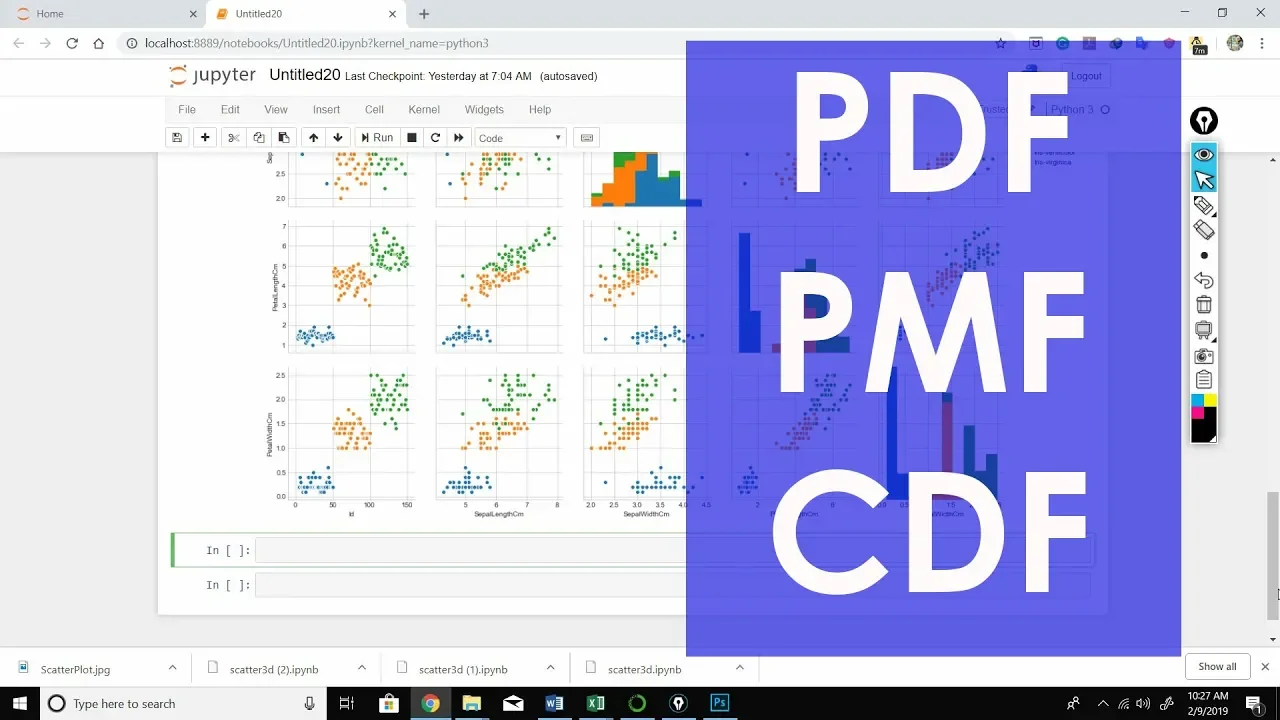




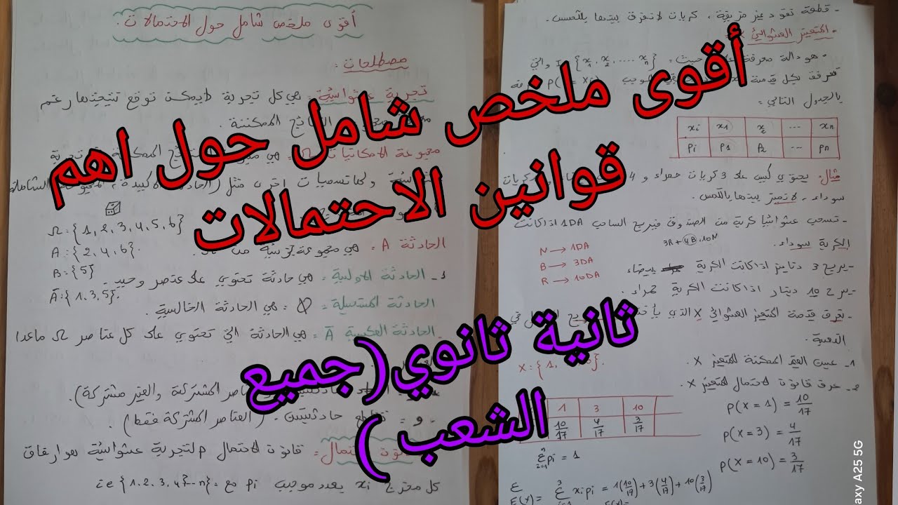


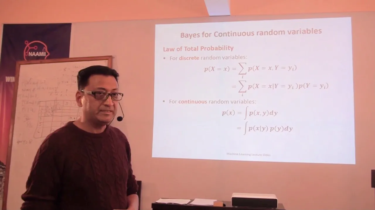
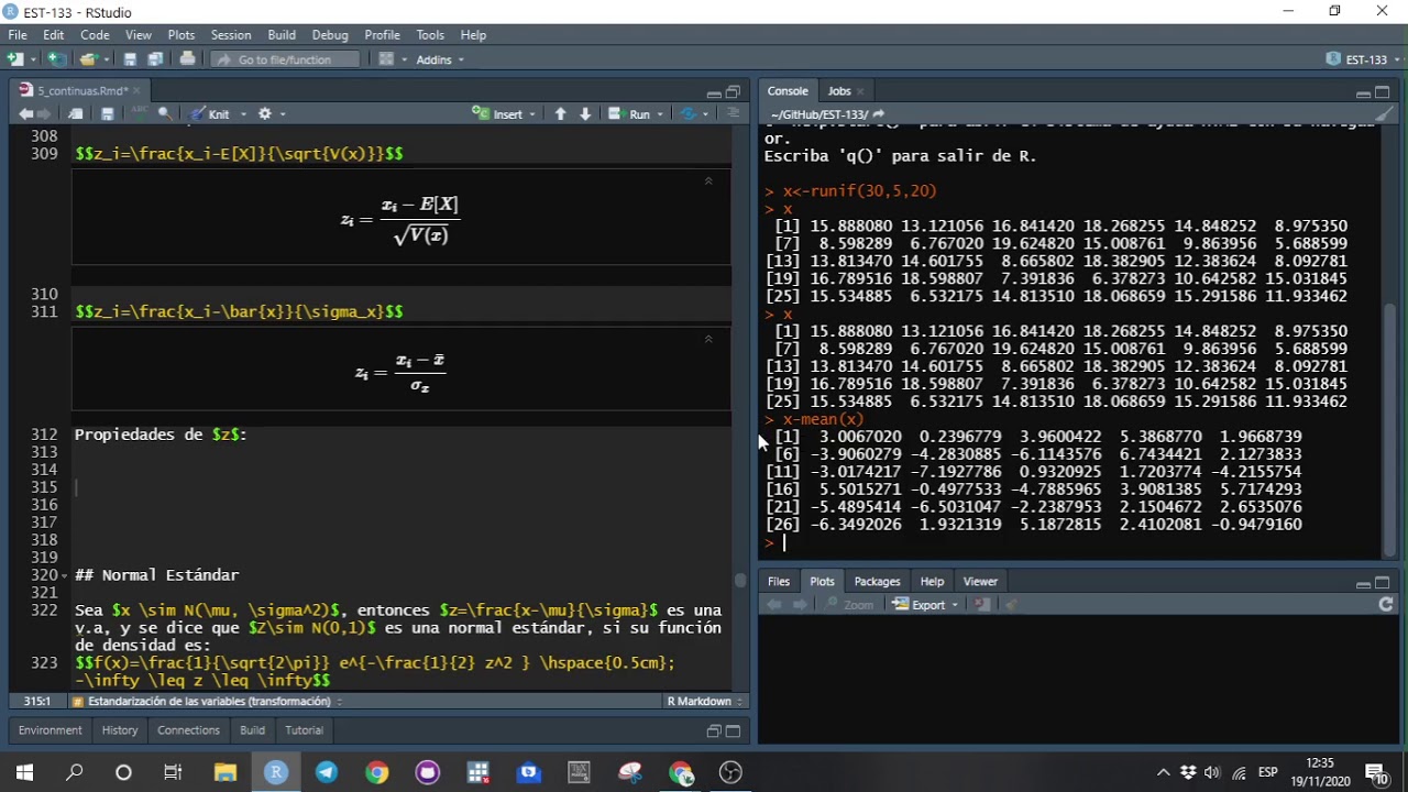


A random variable is a function that maps outcomes of a random process to numerical values, serving as a bridge between abstract events and mathematical analysis; there are two main types—discrete random variables which take on countable, distinct values (like coin flips or dice rolls) and continuous random variables which can take on an infinite number of values within a range (like exact measurements such as rainfall); the probability distribution describes the likelihood of each possible value occurring, enabling quantitative analysis of uncertain events through tools like probability distributions and expected values.
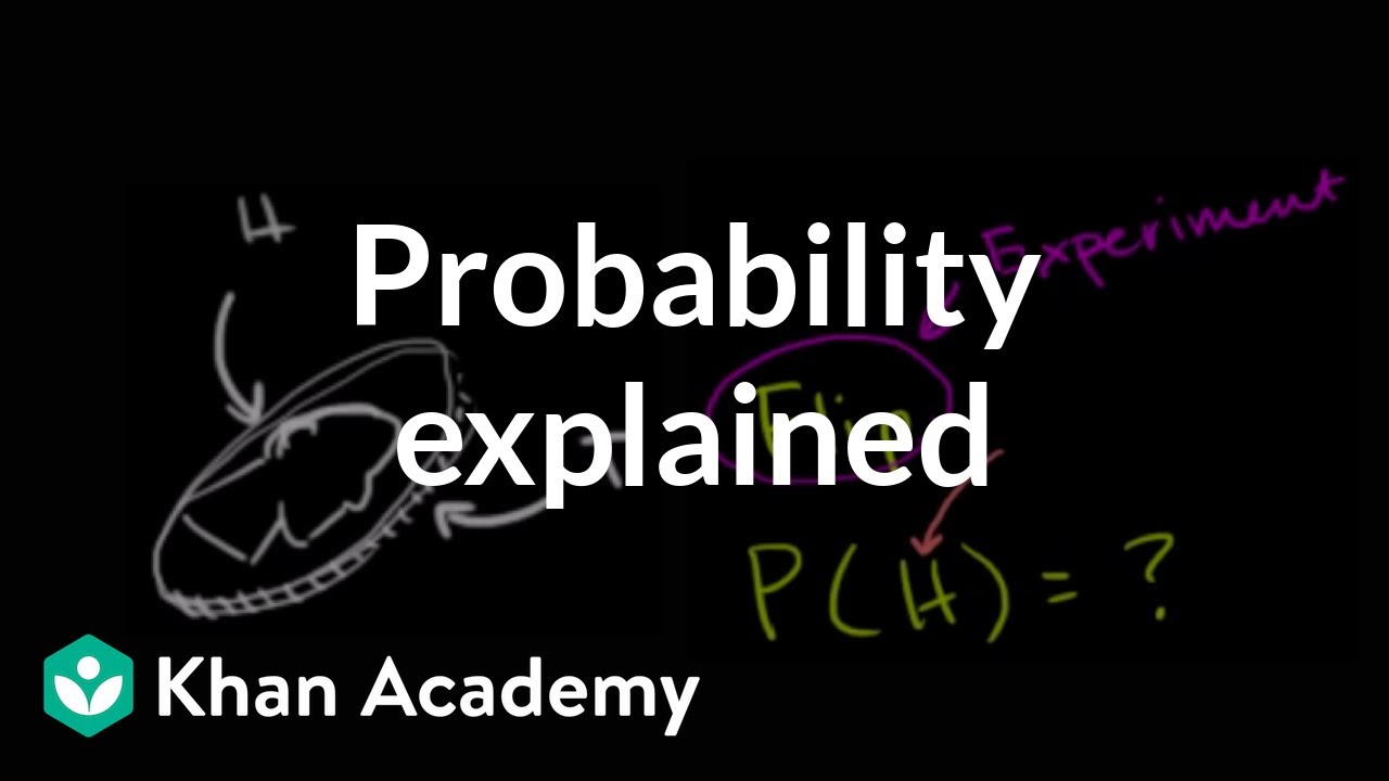
Random Variables Explained: Discrete vs Continuous | Probability
Added:Basic Probability Concepts: Understanding sample spaces, events, outcomes, and how to calculate simple theoretical and empirical probabilities.
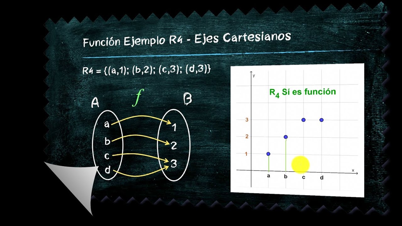
The Concept of a Mathematical Function: Knowing how an input maps to a unique output, which is foundational since a random variable is a function mapping sample space outcomes to real numbers.
Types of Quantitative Data: Distinguishing between countable (discrete) values and measurable (continuous) values in basic mathematics or algebra.
Probability Mass, Density, and Cumulative Functions: Learning how to mathematically represent distributions using PMFs (for discrete), PDFs (for continuous), and CDFs.
Expected Value and Variance: Calculating the long-term average (mean) and the spread (variance and standard deviation) of random variables.
Standard Probability Distributions: Studying specific, named distributions such as the Binomial and Poisson distributions (discrete) and the Normal and Uniform distributions (continuous).
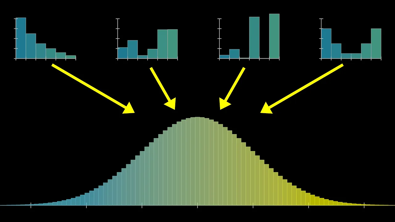
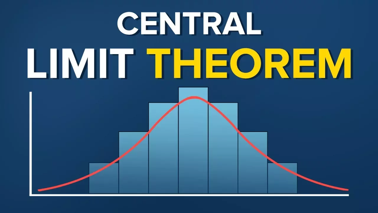
The Central Limit Theorem: Understanding how the sum or average of a large number of independent random variables behaves, which is the cornerstone of inferential statistics.
1.1M views4.6Klikes12:04Original Release: 2009-02-16
I'll now introduce you to the concept of a random variable.
And for me this is something that I always had a lot of trouble getting my head around, and that's really because it's a byproduct of what it's called.
It's called a variable and we're used to variables as kind of an unknown in the equation.
If I write x plus 3 is equal to 7, the variable was x.
Maybe you could solve for it or maybe you could have an equation y is equal to 3x minus 2.
And then, here y and x are both variables.
If you input 1x you could solve for the other variable, y.
And you can change them.
And variables were kind of things that could change and that you could solve for.
And they could take on particular values.
A random variable is kind of the same thing in that it can take on multiple values, but it's not something that you really ever solve for.
So just so you get used to the notation, a random variable is usually a capital letter.
Usually a Capital X, Y, or Z.
Usually a capital X.
And where it really defers from a traditional variable is that it can take on a bunch of different values, like a traditional variable but you never solve for it.
And really, it's a little misleading to call it a variable at all.
It's really a function.
And it's a function that maps you from the world of random processes to an actual number.
So let's say-- I don't know-- I wanted to somehow quantify a random process.
Is it going to rain or not tomorrow?
So let's see-- rain tomorrow.
No rain.
So you could observe that.
You could wait until tomorrow and see if it rains or not, but then, how do you quantify it?
Well, we can define a random variable that will quantify it.
We can say this random variable is going to be equal to 1 if it rains tomorrow and it equals 0 if it doesn't rain tomorrow.
We didn't have to assign 1 and 0; those tend to be a little bit more useful.
They make sense.
But we could have assigned this as-- I don't know-- we could have said that this is 21 and that this is 100.
It's however you define it.
So it's important to keep this distinction in mind, that a random variable-- it isn't a variable in the traditional sense of the world.
It's more of a function that maps us from the world of a random process to a number.
And then, this number is going to be random.
Because we don't know if it's going to rain or not tomorrow, maybe we have some sense of the probabilities.
So this variable can take on either value.
And that leads us-- let me draw a couple of more random variable definitions just so you get the intuition that these really are functions.
So we could define a random variable x as equal to-- well, actually, let me-- It could just be a very obvious numeric mapping.
It could just be the number facing up when I roll a fair dice.
That's a random variable.
I could've also said just the number most facing east when I rolled a fair die, although that's a little less useful.
You could also define a random variable, x is equal to-- you could say it's equal to 1 if heads, and I could say 0 if tails.
Or I could have done it the other way around.
Once again, these heads and tails are outcomes of an experiment.
When I flip a coin that's a random process, each flip is an experiment and then the random variable is just quantifying that experiment.
So I know it sounds a little technical with the terminology, but what we're really doing is fairly something simple.
We're just assigning a 1 if we get a heads, a 0 if we get a tails.
And the random variable is just that function mapping.
Now I'm going into all of this random variable business, which I didn't do before when we did probability because it does start to become a little bit useful notationally.
Because we'll start to talk about things like probability distributions and expected values, and it really is useful to quantify things as a random variable.
And with that said, let's talk about probability distributions and expected values.
So the first thing, probability-- actually, let me define something else.
There's two types of random variables.
You can have discrete random variables, or continuous.
So there's two types.
Discrete would be like, really all of the definitions that we had up until now.
The flip of a coin, you're either going to get a 1 or a 0.
There's two discrete cases.
When I roll a die there's 1 of 6 different outcomes I can have.
Whether it rains tomorrow, there's 1 of 2 outcomes: yes or no.
So in all of these situations you could almost say you could have accountable number of outcomes.
A continuous random variable could take on an infinite number of outcomes.
So a continuous random variable would be the exact-- it could be x is equal to the exact amount of rain in inches tomorrow.
Now why is this continuous?
Well, if you think about it that could take on any of an infinite set of values.
You might have 1 inch of rain tomorrow or you might have 1.1 inches of rain.
You might have 1.111 inches of rain.
You might have 2.1111 inches of rain.
As you could see, you can come up with an infinite number of combinations of the amount of rain you have.
To get exact-- well, I'll go into more of this when I talk about probability density functions.
But in general, even though you might say, oh, well, I can't imagine having an infinite amount of rain because we're not going to have 100 gallons of rain tomorrow.
But if you think about it, you could take on any value between 1 and 2 inches of rain.
There's actually an infinite number of values between 0 and 1.
For any value you could find a number that's a little-- just to think about it.
Between 0 and 1, 1/2 is in between those.
And you can always find a number that's halfway between those and then a number that's halfway between those.
There's an infinite number of numbers between any two numbers.
While, with the discrete random variables, it just took on a finite number of values.
Those ones up here, it could only take on 1 or 0.
It didn't take on 1.1.
Or it couldn't take on infinity.
And I make that difference because actually, how we look at it in terms of their probability distributions are a little different.
But they're very related.
So a discreet random variable like the ones that we had defined at the beginning of these videos, they have a probability distribution.
Let's do it for-- let's say x is equal to the number facing up on a fair dice.
So we already know that to get each outcome-- there's 6 outcomes.
You either can get a 1, 2, 3, 4, 5, or 6 facing up.
So let me draw the probability distribution.
So here are all the outcomes.
I'll draw that on the horizontal axis.
So you get one outcome is 1, 2, 3, 4, 5, 6.
And then, in the y-axis or in the vertical, you plot what is the probability of each of those outcomes occurring?
What's the probability?
I'll switch colors.
So what's the probability of getting a 1?
Well, it's 1/6.
So if I draw 1/6 here.
So the probability is of each of these occurring-- oh, I didn't want to do it like that-- are 1/6.
It's essentially like a histogram or a bar chart.
My intention is to draw them all the exact same height.
So this is telling us that each of these there's a 1/6 chance of it occurring.
If I were to draw a probability distribution for-- if I were to find the random variable x is equal to 1 if heads, 0 if tails.
This has a very simple probability distribution.
There's only 2 outcomes.
You're either going to get a 1 or a 0.
And then in the y-axis you'll have the probabilities.
And each of these, if it's a fair dice, it's going to be a 1/2 probability.
And you're going to draw a little box like that that tells you each of them are 1/2.
Now let's say that you had another-- I don't know-- probably distribution function that looks something like this.
Those are kind of very run of the mill examples, but what if I had something like this?
Let's see.
Where I had some dice-- let's say we had some weird weightings on it where it had an outcome of 1-- I had a 1/6 chance like that.
Let's say for some reason a 2 could never happen.
Maybe there is no 2.
Let's say 3 has a 1/6 chance, a 4 has a 1/6 chance, a 5 has a 1/6 chance.
And let's say there's two 6's.
Like we erased the 2 and we put a 6 where the 2 is, so there's two 6's.
So the 6 has a 2/6 chance.
So the 6 would be a 2/6 chance.
So now I think you can see where the probability distribution function starts to become a little bit more interesting.
In the other ones it was kind of what we would call a uniform distribution.
All of the outcomes are equally likely.
That's a uniform distribution.
Once again, this is a uniform distribution.
This one, all of a sudden, is not a uniform distribution.
1 is just as likely as 3, 4, 5.
2 is impossible to happen, but 6 is twice as likely to happen as everything else-- is 2/6.
If someone gives you a probability density function or if they give you a little chart like this, you can immediately say, what's the probability of different events occurring?
So if you said that x is equal to the number on unfair dice that's described by this probability distribution function.
Then if I were to ask you the probability that x is equal to 6, you'd say, oh, the probability x equals 6 is equal to 2/6 or 1/3.
If I were to say what's the probability that x, the random variable x as given by this definition, is greater than 5, you would take-- well, let's say greater than or equal to 5.
Because you want to include 5, and at least, I did.
So it would include this situation and this situation.
So it'd be 1/6 plus 2/6.
And so you could say that's 3/6 or 1/2.
So it gets pretty interesting once you don't have a completely uniform distribution.
And I'm doing all of this because in the next couple of videos-- well, one, we'll move away from discreet and actually study continuous probability distributions, which are called probability density functions.
And then we'll go to study kind of a lot of distributions that show up in nature.
The uniform distribution is one of them.
There's also the binomial distribution and the normal distribution, which is what some people call the Gaussian or the bell curve.
Which is kind of a very common thing.
But anyway, I'm all out of time and I'll see you in the next video.
Up Next

38:07
Calculus Basics for Quantitative Finance Interviews | Limits, Derivatives & Integrals
@AlanDu-zf8zs
277 views•2023-07-12

4:43
Elliptic Curve Cryptography Explained: ECC, ECDSA, ECDH
@PracticalNetworking
28.5K views•2024-10-21
6:22
Jacobian Matrix Explained | Local Linearity & Transformations
@khanacademy
580.9K views•2017-01-10

6:00
The Mathematical Impossibility of Accurate World Maps
@Vox
23.3M views•2016-12-02
Related Study Plans & Knowledge Roadmaps
Structured learning paths in Mathematics
mathematics
Tensor Calculus: Vectors to Riemann Curvature
01Mathematical Foundations: Linear Algebra & Calculus
02Covectors, Dual Spaces, and Tensor Basics
03The Metric Tensor and Index Gymnastics
+ 2 more learning modules
40h5 modules
Explore Roadmap
mathematics
Gödel's Incompleteness: Logic, Proofs & Limits
01Introduction to Formal Systems & Hilbert's Dream
02Set Theory, Cardinality, and Cantor's Diagonal Argument
03Arithmetization and Gödel Numbering
+ 2 more learning modules
14h5 modules
Explore Roadmap
mathematics
Galois Theory: Fields, Groups & Solvability
01Foundations of Abstract Algebra: Groups & Fields
02Polynomials & Field Extensions
03Splitting Fields & Symmetries
+ 2 more learning modules
24h5 modules
Explore Roadmap
mathematics
Non-Euclidean Geometry: Models & Geodesics
01Euclid's Fifth Postulate and the Birth of New Geometries
02Hyperbolic Space and the Poincaré Disk Model
03Geodesics: Defining Straight Lines in Curved Spaces
+ 2 more learning modules
15h5 modules
Explore Roadmap