










![Mentoring UTS Semester Genap 2024 [Matek-1]](https://i.ytimg.com/vi/Whh_s0XJYic/sddefault.jpg)











The IS-LM-BP model with general functions extends the closed-economy IS-LM framework to open economies by incorporating the balance of payments (BP) curve, which represents equilibrium in the goods and capital markets. The IS curve shows goods market equilibrium where output equals consumption plus investment plus government spending minus net exports, with a negative slope due to the inverse relationship between interest rates and investment. The LM curve represents money market equilibrium with a positive slope reflecting increased money demand at higher incomes and lower interest rates. The BP curve captures balance of payments equilibrium, where the current account (improved by currency depreciation and worsened by higher GDP) and capital account (attracted by higher domestic interest rates relative to world rates) must balance. The model's three curves intersect at a unique equilibrium point when the Jacobian determinant of the system is non-zero, enabling comparative static analysis of how government spending, money supply, and world interest rates affect equilibrium income, interest rate, and exchange rate.
IS-LM-BP Model with General Functions: Introduction
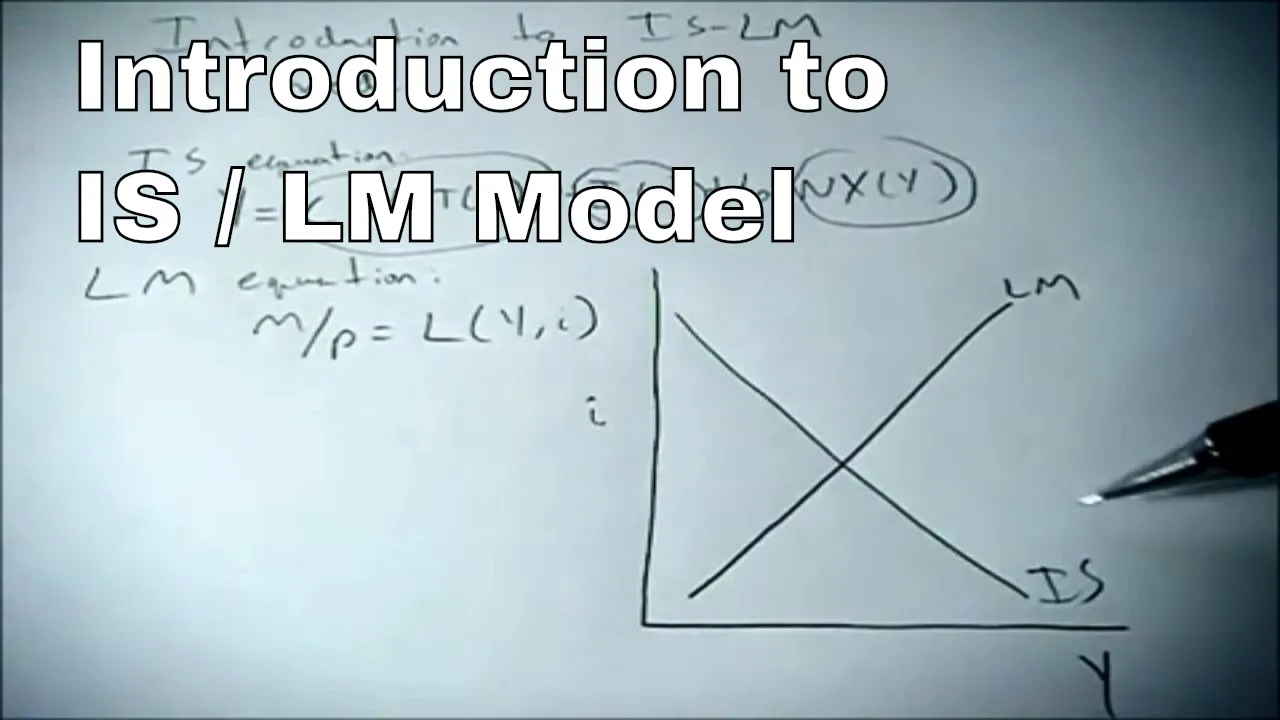
Added:hi in our previous video we've covered i7 model with general functions so now we are moving to isl mp as i told you before due to the fact that we are using now general functions all calculations of comparative static derivatives are going to become way easier however at the beginning we of course need to do some ground work to derive every element of the model and let's start as always with eyes curve but here actually as you see the setup is almost identical as in the previous just isi model except we are adding current account current account is simply net expense and here you see we are assuming that current accounts have two determinants first one is exchange look we already said that assuming that exchange rate is defined how many units of our currency we need to pay for one unit of foreign currency right in this case higher exchange rate means depreciation right and with depreciation we know that our goods are becoming more competitive and because of that current account improves so based on that we can say the partial derivative of current account with respect to exchange rate is positive so the more we need to pay for one unit of foreign currency the better should the very should be our position in the current account pass balance on that trip of course current account has a second determinant which is a gpu now here we're actually talking about npi marginal compensation import we're going to define uh denote this as c a y and we know that this must be lower than zero and look because this is npi right so we can say the absolute value of this should be [Music] zero and what but this is not the most important thing the most important thing are those two relationships you know that actual depreciation improves current account while higher gdp due to the fact that we spend more money on imported goods has negative impact on the current account okay so um so uh carrying on carrying on this is truly the only new things new thing we've got here in comparison with isl mvp with islam model we of course remember that derivative of consumption with respect to disposable income which we are denying c prime is our marginal propensity to conceal and somewhere between 0 and 1 we know that the derivative of taxes with respect to income is a tax rate which is also between zero and one and we remember that in order to differentiate this expression with respect to income what we need to do is to use the chain rule right you know but over here the intermediate step between income and consumption is disposable income so yes this is equal to c prime times the derivative of disposable income with respect to income which is one minus t prime into just one single equation that is going to be now first thing we should do knowing that this is our new is curve is to try to estimate its flow right so [Applause] first thing we do of course we differentiate this expression with respect to income and interest rate right in this space we are actually drawing uh the is curve okay so how does it uh so how does it we've got ui uh equals to c prime times one minus t prime d y plus i prime o that was one thing i hadn't said but it's just like we had in the previous case that of course derivative of investment with respect to a interest rate is of course negative the higher the interest rate the lower now okay so we've got i chronium then we got plus nothing right because uh this doesn't contain either income interest rate and out of this one we've got income over here we'll have that this is c-a-y okay hello let's do it like that let's put all the expressions uh with y on the left-hand side and everything else finally on the right hand so we've got one minus c prime one minus t prime minus c [Music] now dividing both sides by d y and i prime we get that d i over d y is equal to 1 minus c prime times 1 minus t prime minus c a y over i prime now what do we know about it what do we know we know that this part is somewhere between zero and one we know that this expression is negative consequently minus and minus this is plus we know the p upstairs is positive and finally this derivative is negative so positive and negative pieces negative we know that is curve is going to be downwards slowly so in that income interest rate space the ice curve is gonna be downwards so now we move to lm curve actually lm curve is going to be no different than the one that we have in case of island model with general functions but as you remember i hope you remember we had we had exactly the same situation when we were dealing with vulnerable so it shouldn't come as a surprise so we've got money demand equals money supply as equilibrium condition money demand is given as f y i where we know that derivative of modern demand with respect to income which we defined as l y is positive well derivative of one demand with respect to interest rate which we defined as delta i is located and again we are also assuming that money supply [Music] is given by in this case we get that the entire number could be condensed into one equation and in order to get slope of the line we need to differentiate with respect to income and interest rate so we get l y y plus l i d i equal to zero once we rearrange it [Applause] and divide both sides by d y and l i we get the slope of lm which is equal to negative m y l i and you of course remember that because f i is negative and y is positive and minus in front it must be bigger than zero now we are finally ready to add i'll refer to our graph okay and finally the only curve left we've got is we already discussed final points of it when we were discussing [Music] when we were discussing the lunar model so it also should go pretty fast but now we've got bonds of payment curve and once the payment curve is defined in a very similar way because we get it with the linear ball this is the sum of current accounts and capital account but let's denote this capital account here because there would be again too many uh too many things of course if exchange rate is supposed to be equilibrium those two must be closing at zero now we redefined ca already as a function of exchange rate and income we already established that the two derivatives are cae which is positive depreciation improves current account and see why it's negative higher income means higher imports and worsening of off trade packets however now we've got also capital account function and similarly to what we had previously capital accounts is going to be a function of domestic and world interest rate and look here again we need to define appropriate derivatives so partial derivative of current of capital account with respect to interest rate which will denote ki must be positive what does it mean if interest rate in our country goes up while interest rate remains uh the same in the rest of the world our assets become relatively more attractive and uh people from the rest of the world like to purchase our assets so they will need to purchase our currency in order to purchase our asset so our country actually experience capital info and look reverse must hold for the word interest rate it needs to be negative why well while holding now domestic interest rate constant if inch or the interest rate goes up it means that foreign assets are becoming more attractive now home residents domestic residents need to purchase foreign currency in order to purchase assets dominate foreign assets denominated in foreign currency so we will see capital alpha okay and look this is enough for us actually to have the bb curve so now let's calculate the slope of vp well again we just need to use the equation we already have and differentiating respective income and interest rate okay so we've got c a e y plus k i i equals we differentiate it uh with respect to income and interest rate so we get this c a y [Music] again we move this to the other hand side we divide both sides by d y and k i and we get the slope of bp to be negative c a y over k i now k i is positive c a y is negative minus a prime so this expression must be positive so look we've got the third curve the bp curve that is upward slope however let's notice one thing we've got two curves there are upward sloping lm and pp so why did i draw it like this well i draw it like this because let's just say in reality high capital mobility is something that is true for most countries so bp is generally fatter than allah however now that we we are able to analyze this model using simpler arithmetics because we use implicit function rule and it's easier for us to calculate comparative static derivatives we will be able to actually assess what happens if b b is more steep than but this a little bit later okay our next step is of course to assess the complete model oh so we're going to have three curves first is an ice curve where this is a function of three endogenous variables income interest rate and exchange rate and in our case this is also a function of three exogenous variables government spending money supply and work interest rates now how should we write it well we should use we need to express it as equals to zero so we use the equilibrium condition and we write it as y minus c y d minus i i minus g 0 and minus c a e and this equals zero okay then we need to take care of the lm curve we also treat as a function of income interest rate exchange rate and three enzymes variables g zero and zero and i die now here's a situation simpler with vectors l y i minus m zero equals to zero now finally the bp curve which we also write as a function of income interest rate and exchange rate three endogenous variables and three x generate g o m zero i w and it's equal to c a so now what is the first thing we are doing in this case we need to see if those three functions are actually defining and implicit functions of exchange rates the income interest rate and exchange rate as functions of uh exogenous variables now so we need to calculate digital right and if jacobian is different than zero then we know that this is true and we know that the equilibrium in the model that we want to analyze so again we start by calculating the jacobian and how do we do it just like you did before remember here we've got first function second function third function we need to differentiate them with respect to endogenous variables so first we differentiate with respect to y then with respect to i and then with respect to e so income interest rate connection so let's go out of the first one if i def differentiate with respect to income i'm gonna get this this is one minus c prime one minus t prime minus c a y okay i'm gonna make it bigger okay then if i'm gonna differentiate the first equation now with respect to interest rate i'm gonna get negative i try and reduce back to exchange rate i'm gonna get negative ca e okay then we're gonna do it for the second equation if i'm differentiating it with respect to income i'm getting alpha interest rate i action drink two there's no action and again now we differentiate the third equation with respect to income so we can see why interest rate ki and exchange and let's do this very simple thing first thing i can do with this chakra is i can take c a e remember this trick is very important with all the calculations and makes everything simple okay so we've got one c prime one minus t prime plus minus c y now minus i prime minus c a e and uh minus one then we got l one l i zero c y k i y okay and the best way to do it actually is to use one class expansion okay so what do we get we have c a e in front we open fractions okay so i'm going to expand it using the last part so this element first of all so we got just negative one in front of if i'm deleting first row third column this there is this element it's just one it lies in the third row third column so we don't change the sign and you move it like this by one minus c prime y minus t prime minus c a y minus i prime l y l so now we can calculate this all the way through and we get negative that this is negative my ki minus c a y alpha but there's minus up front so it's plus right minus minus now we are dealing with this part so we've got plus one minus c prime one minus t prime minus c a y times l i and now plus l y times n okay and this is look we can easily see that here we've got uh we can easily see that we've got c a y and i the plus and c a y those cancel each other out and we see that both of those fly so we can put them together okay let me just finish this over here and based on what we calculated we get c e and now times uh one minus c prime y minus t prime times delta plus ly times i prime minus k i okay so now we have found the expression for the jacobian we need to assess itself we know that this is between zero and one we know that this is negative so those two together are negative now look this is positive this is negative this is positive however if his mind is a fraud right so this is negative times positive this is also negative and cd is positive right the depreciation leads to improvement of current account so we know that the chocolate gun is lower than zero and because it's lower than zero it's different so because we know that the jaguar is different than zero we can proceed with our law and look what what do we get first we can finally write that those three curves intercept at one given point and on the graph this point is going to give us in income interest rate but also exchange that we simply do not see because this is just two-dimensional model but there is equilibrium interest rate uh extreme rate associated with that law and look what doesn't mean for us is that now we know that these three functions above are defining three implicit functions so income as a function of government spending money supply and board interest rate interest rate equipment interest rate as a function of government spending money supply and a world interest rate and finally exchange rate as a function of government spending money supply and work interest rate right but look this is actually also allowing us to proceed to the next step because knowing that those and knowing that those are implicit functions and they are identities at the point of evaluation [Music] we can rewrite the system that we had over here again we can write is y minus c y d minus i as a function of equilibrium interest rate minus g zero minus c n as a function of equilibrium exchange and equilibrium and we know that this is equal to zero now i can do exactly the same thing for allah and i can do the same thing for pp okay so what do we do next well in the next step what we are going to do is to differentiate all those three equations okay so again we start with is so we've got okay we already know more or less we already differentiated it so i'm going to make it a quick step this is going to be 1 minus c prime 1 minus t prime minus c a y right times d y then we will have minus i prime d i and minus [Music] and of course exogenous variable minus uh now we move to a lab your situation is simple l y d y plus l i d i o minus d and finally the last equation we've got c a e d e plus c a y [Music] okay so what should we do in the next step well of course in the next step we will organize the variable so all that endogenous variables goes left hand stay on the left hand side generation moves to the right so we've got one minus c prime y minus t prime um minus c hey i'm sorry minus minus uh [Music] minus a plus plus ki and this is equal to this is our only exogenous variable okay and look i hope you can see that at this moment we are ready uh we are ready to put this system into matrix notation okay so to start with matrix of coefficients uh matrix of coefficients uh one minus c prime one minus t prime [Music] minus [Music] our uh endogenous variations so the differentiator d i d y d i and d e [Music] iw and now we're ready look what have we done we've derived islam mpp we found a jacobian of course we estimated we evaluated their slopes we've calculated the jacobians so we know they intersect in one place we know that equilibrium solutions are available so we will be able to find comparative static derivatives and this is the system of simultaneous equations that we're gonna use for it so the only one thing left is to analyze the impact of government spending money supply and work interest rates on equity bloom income interest rate and exchange this is going to be a topic of our next videos okay thank you for your attention and in the next video we're gonna analyze impact of monetary policy in this model
Up Next

IS-LM-BP Model: Open Economy Macroeconomics Tutorial
@AddingtonCoppinECONOMICS
41.3K views•2015-03-20

Impact of Yuan in Indo-Russian Trade Amid Sanctions
@WION
261.9K views•2022-07-01
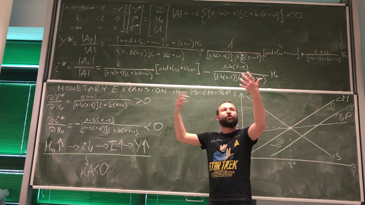
Monetary & Fiscal Policy in Open Economy IS-LM-BP Model
@lazarskiopencourses4059
559 views•2021-04-11

The Age of Easy Money: Fed & Inflation | Full Documentary
@frontline
21.2M views•2023-03-15
Related Study Plans & Knowledge Roadmaps
Structured learning paths in Economics