









![สถิติและการแจกแจงความน่าจะเป็น ม.6 - ปูพื้นฐาน [Part 1/2] | คณิตศาสตร์ By พี่ปั้น SmartMathPro](https://i.ytimg.com/vi/VKblxmZfJ58/maxresdefault.jpg)

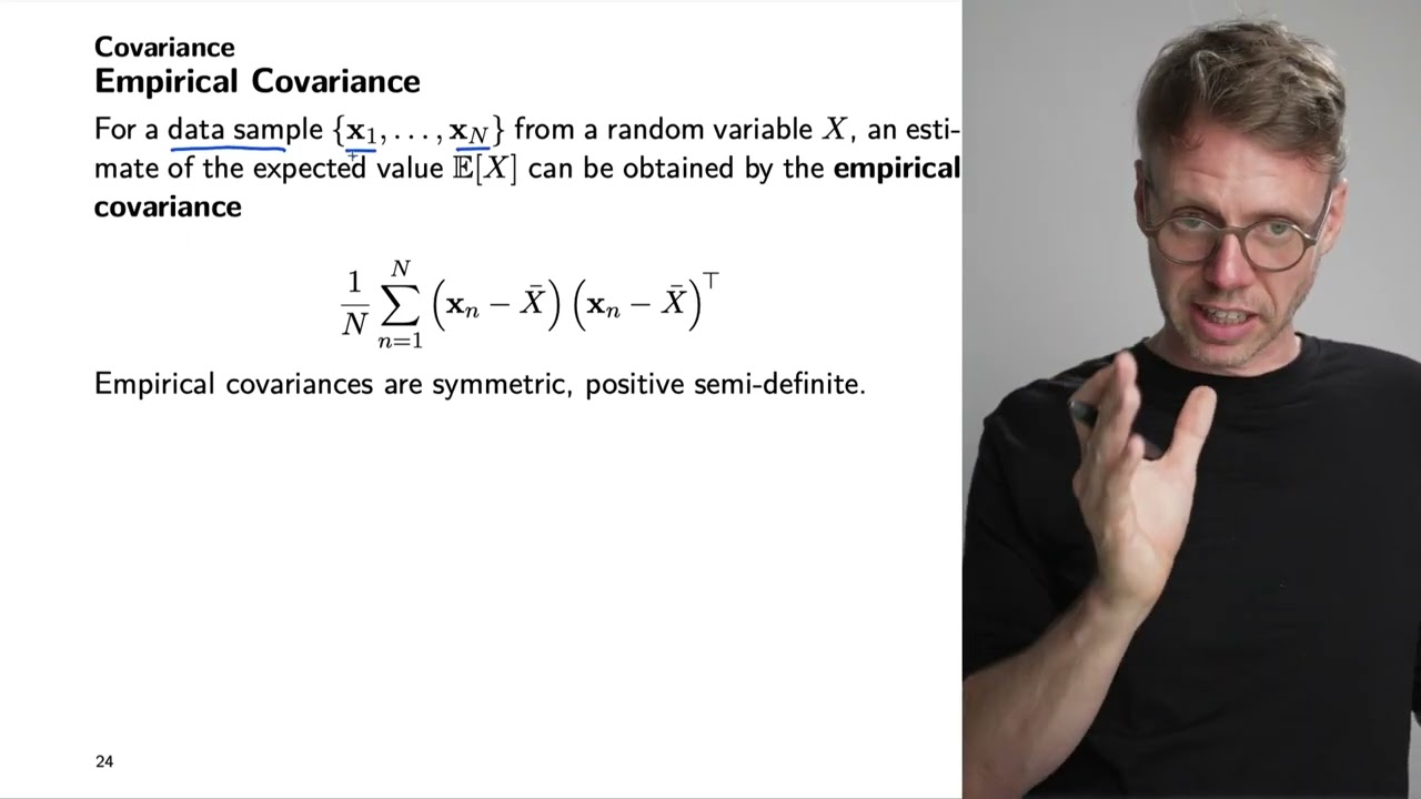







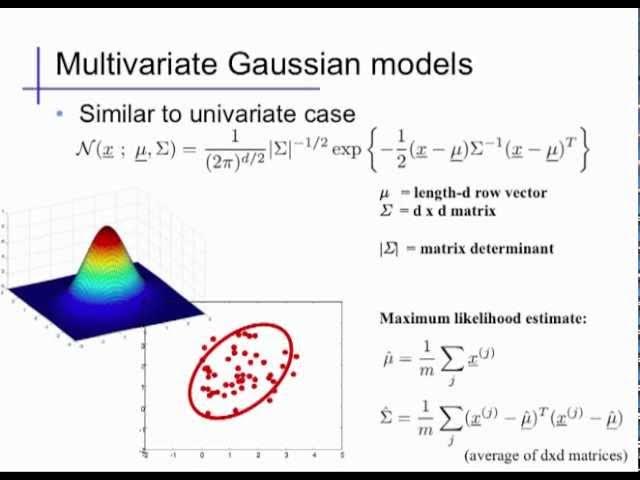




In machine learning, we optimize by minimizing 'surprise' (the negative logarithm of probability) rather than probability itself, because surprises transform complex probability distributions into simpler forms (like polynomials for Gaussians) that align with linear algebra operations, making computation tractable; this approach connects probability theory, linear algebra, and calculus through the Gaussian distribution, which emerges naturally from the Central Limit Theorem and simplifies to quadratic forms that computers can efficiently solve.
Probability Fundamentals for Machine Learning | Math4ML Guide
Added:Basic Algebra and Functions: Comfort with logarithmic functions, which are crucial for understanding surprise and information functions.
Introductory Calculus: Familiarity with the concept of integration and the area under a curve, essential for understanding continuous probability density functions.
Set Theory Basics: An understanding of sample spaces, events, unions, intersections, and Venn diagrams to build basic probability intuition.
Descriptive Statistics: A fundamental grasp of measures of central tendency and dispersion, specifically mean, variance, and standard deviation.
Information Theory Foundations: Exploring Shannon Entropy, Cross-Entropy, and Kullback-Leibler (KL) Divergence, which build directly upon surprise functions.
Bayesian Probability and Inference: Applying probability fundamentals to Bayes' Theorem, prior/posterior probabilities, and Maximum A Posteriori (MAP) estimation.
Multivariate Distributions: Extending univariate Gaussian concepts to multivariate Gaussian distributions and learning how to work with covariance matrices.
Probabilistic Machine Learning Models: Studying algorithms that leverage these probabilistic concepts, such as Gaussian Mixture Models (GMMs), Naive Bayes Classifiers, and Variational Autoencoders (VAEs).
36.1K views807likes45:05Original Release: 2021-01-14
[Music] hopping back in to it directly a reminder of the overall themes structures goals of this webinar series the overall goal is to understand what math has to do with machine learning and even though all programming involves math at some level in some way we can always use the tools of mathematics to understand the programming that we're doing machine learning because it's programming by optimization really benefits from some strong grounding in mathematics and so we're using the tools of mathematics to understand that optimization process that goes on during machine learning there are basically three core ways that optimization and machine learning intersect in terms of the objects being optimized in terms of how we optimize and in terms of what we optimize we already talked about the objects being optimized by using linear algebra to understand that data and models are arrays and linear operations on arrays is linear algebra and it's a part of the core of machine learning then we understood how we optimized with calculus which means we basically make tiny changes using this framework of linear approximation and then finally now we're going to understand just what it is exactly that we are optimizing very loosely up to this point i've said that we're improving the performance of our model but that's not very quantitative at all and so we're going to see that actually what we're optimizing is we're reducing the surprise or uncertainty of our models when they're presented with data and so the tools of probability and statistics are going to come in very much handy here so let's dive in and talk about probability the bad news i have here is that even those first two sections we talked about linear outro when we talked about calculus there's i think a lot that's intuitive about these ideas they're relatively easy to work with there's some subtle ideas but once you wrap your head around core ideas like arrays and approximation the world is your oyster but probability on the other hand is surprisingly subtle in a way that makes it very difficult to work with so bertrand russell who is one of the premier mathematicians and logicians of the early 20th century said that no one has the slightest notion what probability means and bertrand russell was very fond of paradoxes but he liked them to be a little bit neater than the paradoxes that you find in probability another indication of just how subtle and difficult probability can be is this quote from probability and introduction a textbook by samuel goldberg which notes that the concept of a random variable which is at the very center of probability we say oh this is a random variable that's a random variable is actually a tremendous misnomer so just like an alligator pair which is neither an alligator nor a pair a random variable is neither random nor variable an alligator pair is actually an avocado it's an old name for an avocado and that's not a type of pair uh and the random variable and probability is actually a deterministic function but it's the way things are termed and that suggests that there's something we want to treat it in one particular way this random variable idea that we have this intuitive idea when it comes time to turn into mathematics things get complicated uh and then finally i've often in the last two sections mentioned content by three blue one brown who's one of the premier math youtubers these days three blue and brown attempted to make a probability series and then eventually gave up they were working on it they got about halfway through it and then they realized you know actually there's a lot of ambiguity in what people mean when they say they want to learn probability and so they gave up on that plan that they had probability is something of a white whale in mathematics like in moby dick it's a difficult idea to try and conquer we aren't going to be totally dismayed by this and give up entirely but i just want to put that out there just as an indication that this is the hardest of the three sections uh and so i'm gonna try and present as much intuition and ideas around probability as i can but you shouldn't be surprised if this one is a little bit maybe less satisfying more difficult in some ways but when i say probability surprisingly subtle the there's some parts of this that go all the way back to like what does it mean what are we even trying to mathematically model here before we go out and write our definitions just as an indication of this difficulty let's consider the expression pi of n which just means the nth digit of pi so when i say pi one i mean three when i say pi of two i mean one pi of three is four and so on all the way through the digits of pi and so the quantity d equals pi of one that's just the number three and if i ask you a question is d even or odd it's pretty straightforward to know how to answer it d is three that's an odd number and if i ask you what is the probability that d is odd before we dive into definitions or think too hard about this so you have a clear intuitive answer in your head it's three it's odd 100 chance that it's odd there's no chance that it's not odd the difficulty comes in when we do something like consider the quantity pi of 4.65 times 10 to the 185th so this is roughly if i were to write a single digit of pi on every single tiny scrap of the universe every single planck volume this is how many digits of pi i could write out so no one will ever be able to write out pi this far unlikely anybody will ever be able to calculate it this far and we don't know what that number is so question i have for you is which of the following would you say is a more correct way of thinking about it to say that d is even with probability 0.5 there's a 50 50 shot that d is even or to say that d is either even with probability one or zero but you just don't know which of those that is so this one is is more of an opinion poll than it is a mathematics question and one thing i'd like to note here is that so far as we can tell there is no real pattern to the digits of pi every digit seems to occur with equal probability in the long run all right it looks like a consensus is emerging here people are agreeing on one of these two answers uh and one of these is the minority response here so let's go ahead and thanks to everyone who answered let's go ahead and reveal what those answers were all right it seems like the most popular choice here is d is even with probability 0.5 but there's a strong minority of about a third to about a quarter who say that actually no it's the d is either even with probability one or zero but i don't know which interestingly whenever i run this with a different group of students i actually get slightly different answers so i've sometimes seen people like split basically 50 50 down the middle for both of these sometimes i see a result more like what we're seeing here where it's two to one for the first answer essentially these two different answers come down to whether you want probability to mean oh i don't know what this value is and i want to be able to represent my uncertainty about about certain values and then that gives you the first answer or whether you want probability to be this mathematically definable thing about frequencies if you really think okay probability should represent the frequency with which events occur then it doesn't make sense to say that d is even with probability 0.5 there's no sense of frequency in which we can generate pi many times and get different values and so that second approach is the frequencies approach to probability and the first approach is the bayesian approach to probability the first one is a little bit more popular these days it's especially popular in machine learning and popular among practicing scientists but the latter is actually more popular among people who do probability rigorous mathematics of probability so in the end it's something of a matter of taste but the fact that there's a matter of taste at the very beginning when we define the concept that gives our field its name of probability theory should suggest some of the the complexity and difficulty that comes in but we are not going to be daunted by that complexity and that difficulty we're going to proceed forward and just look at what happens without trying to interpret what probability is just looking at turning the crank what do we see and we're gonna have three basic takeaways the first is that if we ignore all this all these questions about what does probability mean mathematically probability behaves just like mass which is something that we don't think of as that paradoxical or that difficult but then when it comes time to do machine learning a related concept called the surprise shows up more often than negative logarithm of the probability rather than probability itself and then finally when we want to use probability distributions when we want to use probabilities in machine learning we most often end up using the gaussian distribution or the bell curve and gaussians end up actually at the intersection of all three of the fields we've talked about of probability linear algebra and calculus but especially at the intersection of probability in linear algebra so we'll talk about gaussians in detail so first what is probability probability is something like mass we use the same mathematical tools that we would use to work with masses with objects that have weight so consider to understand this analogy or this relationship consider the distribution of mass on two pizzas so one pizza is a cheese pizza and the other pizza is a pepperoni pizza i wanted to tell you where is the mass on this pizza well there's a whole bunch of different points right on this pizza there's an x and a y coordinate for every point on this pizza at a given point there really isn't any mass if i ask you at the exact center of the pizza how much mass is there the answer is basically zero at a fixed exact point if i want to know how much mass there is in a part of the pizza what i need to do is i need to integrate over an area i need to say okay there's a little bit of density here there's a certain amount of grams per square centimeter in the center there's a certain amount of grams per square centimeter at the edge and i need to integrate those so i would have some density function for the pizza a pizza density function that says at this point the density is equal to this at another point it's equal to this other value and when we work with masses and densities especially in a typical educational context all the way up to the point where you're maybe in an advanced physics or engineering class you only work with things that have an even density function so if i want to talk about the math of this cheese pizza it's really simple because it's flat and so i don't really need to think explicitly that what i'm doing is an integral i just take the area times some fixed value that we call the density of the pizza and that gives me the mass in any given area and so i can answer any questions about the mass of this cheese pizza the center of mass things like that without having to think too hard about integrals but if i have something like that pepperoni pizza on the right hand side here there's more mass in certain places there's a couple of pepperonis overlapping in the middle so there's a spike in the density there because if you look at any given point on that pizza right there there's more stuff there's several overlapping pepperonis and then as we go to the edges there towards the places where there's only cheese things flatten back out again and so if i want to know how much mass there is in any given point on this pepperoni pizza i actually have to think about okay what is my pizza density function and how much mass is there in this area if i want to know the mass of a part that's say got a pepperoni on it i need to integrate in the area of that pepperoni so this is not that dissimilar to the distribution of dart throws in let's say two separate cases one is somebody who's been blindfolded throwing darts at a dartboard their darts let's say end up everywhere so they throw the darts many times and we look at where the dart ends up and there's lots of darts spread throughout the entire dartboard but if a pro player throws darts at a board and we collect those over time maybe throughout a whole bunch of games we'll see that really often they throw towards the center so that's a very common place for the darts to end up and then other times they throw towards different spots there's a ring in the dartboard there's actually two separate rings of the dartboard that give different amounts of points and sometimes in a game of darts you really want to hit one of those so pro player will have a very complicated distribution of dart throws a complicated spread of darth bros so if i have them throw darts at the board for a really long time then i'll end up with a distribution of darts on that dartboard i can imagine what is the density of darts on this dartboard so i think of that basically as the chance that any given dart ends up at any given spot and much like there's no mass at any given point on a pizza there is no probability at any given point on the dartboard any exact specific precise point that you say oh did a dart land here on the dartboard the answer is zero it's only when we integrate over an area that we can actually get an actual mass in the pizza case or an actual probability in the probability case so what we're mapping here is a density of probability how much probability per square centimeter is there and when we integrate over squared centimeters we get probability just as when we integrate a density of grams per square centimeters we get grams in the end and i think this distinction between probabilities probability densities probability masses this is something that definitely confuses people and i like whenever i get confused by this to think okay what if i were just thinking about math how would this look so this probability density function that describes where things are more likely to end up is the core object that we think about in probability theory the most common thing that we think about so there's a lot of similarities between mass or density and probability we have a density function in the former case that takes a position and returns a real number that is the density and in order to get a final mass we integrate over an object so if i want to know the mass of an object which might be say a slice of the pizza or an area in the pizza i need to integrate the density over that object which looks like the thing on the left it's maybe an unfamiliar way to present a familiar idea of calculating or thinking about the mass of an object that is transferred directly over to probability we have a probability density function that takes in an outcome space now rather than spatial coordinates and returns a real value that is the probability and just like density actually probability is non-negative you can't have negative mass and you can't have negative probability and when you get the probability of an event say the dart lands anywhere in the bullseye or the dart lands anywhere in the inner ring or the dirt doesn't hit the 20-point region then you need to integrate that probability density over that event so even though there are similarities and maybe formally at some like galactic level of abstraction they are the same thing to study density and to study probability with one single tool but there are some differences in emphasis one is that the total probability is always one so if i integrate over the entire dart board the value will always be one if i'm integrating the probability but a pizza need not weigh the same as another pizza there isn't that restriction and that's that becomes very important when we're working with probability we also care quite a bit about the concept of independence in probability which is to say that if i have some function that takes two arguments so a probability of two events maybe can i think of that as just the product of the probabilities of the individual events can i think of these things independently or separately from one another can i factor p of x y into p of x times p of y that comes up all the time in probability and very rarely in calculating masses then finally we care about expectations in probability the expectation of a function is to say okay what if i were to take the outputs of that random variable and i would put them into a function what would the value on average be if i take say the outputs of a random variable i pass them through a function and i take the mean one over n times the sum of the values what would what should i expect that value to be that is the expectation so as an example maybe we want to know what the average score of a pro player versus a blindfolded individual is going to be so i take the position that x and y value here and then i pass that through the scoring function that says okay what is the score that you get for landing in that particular spot and then we could calculate an average score again by means of an integral so this may be heartening to say oh masses are actually something that's pretty easy relatively straightforward so probability should be easy and relatively straightforward but the trouble is that actually when you really start to work with it the math of distributions is really gnarly this math of distributions is also known as measure theory and it's something that even people who do phds and statistics struggle with and find maybe to be an impediment more than a help to their understanding of probability uh so that's a link there to andrew gellman's blog and a discussion of whether measure theory should even be taught to stats phds and one of the fundamental reasons why is that integrals are hard and derivatives are easy relatively uh so when i want to calculate an integral of something calculating it can be basically infinitely difficult uh whereas derivatives can be done automatically by computers as we saw during the calculus section and then finally we have to watch out for paradoxes so there's a famous banach tarsky paradox which is pictured on the right hand side here which is that if you're not careful with defining what it means to measure something and get its size then with a just basically intuitive definition you might end up with a circle that you can then break apart into pieces where when you combine those pieces back together the measure of the total has doubled you've got two copies of the original when you combined it back together so that's a really gnarly paradox and people work really hard to measure measure theory to avoid things like that and this is all separate from those philosophical issues that ident identified at the beginning what does it really mean to talk about probability even once you've solved that you have to solve these more mathematical paradoxes here this is bad news it means that it's actually really hard to get a fully completely rigorous mathematical accounting of what is going on when you talk about probabilities distributions expectations and so on you open up a whole big can of worms when you try and be completely rigorous we have to be a little bit more intuitive when we talk about probability unless we're willing to really dive in and understand that measure theory which is a long and lonesome road uh so we're gonna go in an intuitive direction here and focus on what can we understand without diving into that stuff so we're going to focus on the concepts and ideas and probability that trip the most in machine learning and in particular one that i want to really talk about is the concept of surprise and so surprises show up more often than probabilities in machine learning surprises are inverse probabilities and they're at the foundation of information theory so at again an intuitive level surprise is closely related to probability if something is a little bit less probable it happening is a little bit more surprising uh and if something is certain then it happening is not at all surprising if somebody tells me that two plus two is four then i'm not surprised at all we could say that i am zero surprised if we were looking to quantify it whereas if something is impossible then it happening is more surprising than literally anything else and so if somebody say told me that two plus two was equal to five that would be more surprising than say getting a thousand heads in a row that's unlikely but it's not impossible two plus two being equal to five that's completely impossible so there's infinite surprise when something impossible happens there's zero surprise when something certain happens and then everything else is in between so the difference between probability and surprise apart from this sort of flipping around is that if two unrelated surprising things happen we add the surprises instead of multiplying them so the probability of two unrelated surprising things say getting 10 coin flips in a row right now and it's snowing in beijing right now i would multiply those two probabilities together whereas if i were to take the surpri the quantitative surprises involved in those two events i would add them together if i take just to stick with coin tossing again coin flipping and dice rolling was the earliest thing handled by probability back in the 17th century so people like those examples if i'd if i take the probability of two heads that's one half times one half and that's one fourth if i take the surprise of two heads i add those two numbers together we'll see in a second that it's one bit of surprise to get one head and one bit to get another head that's two bits so together those desiderata or those properties define the surprise as a function of the probability so the surprise of an event is the logarithm of one over the probability of the event which is the same if you remember your logarithm rules as the negative logarithm of the probability of the event this is also known as the surprise zoll there's a couple different names for it if there is a probability density function there is essentially a surprise function defined on the possible outcomes of our random event and we can get it from the probability distribution just by taking its negative logarithm you can also just write down a function subject to a few simple constraints and then that will turn into a surprise which makes it a little bit easier than writing down a probability distribution there's more constraints to write down a probability distribution there's a close connection between this surprise function and the entropy which is that the entropy which shows up in information theory is the expected value of the surprise so if i take the surprise function for a given random variable maybe if you wanted to imagine what this would be to simulate take a whole bunch of values from this random variable calculate the surprise and then look at that average value at the end that will give you the entropy so the negative logarithm of the probability weighted by the probability that's the entropy so surprises are measured in bits which means you can rigorously and quantitatively say that one thing is a bit surprising the entropy shows up in information theory it tells you a lot of things in information theory one of the things it says is how difficult it is to compress something uh and so things that are more surprising that more often produce surprising values are things that are harder to compress that's the core idea at the center of information theory from this idea of surprise we can derive the most common process for doing machine learning by basically doing a competition to see who can be the least surprised by an outcome before it happens we write down how surprised we would be for each outcome before it happens so let's say we're betting on a presidential election a sports game something like that we each write down okay if this candidate wins i would be this surprised if this candidate wins i would be like this other amount surprised if this team scores 100 points i would be this surprised if they score 101 points i would be even more surprised by writing down this surprise number for each outcome we've effectively given a model that says this is more likely this is less likely you're allowed in this competition to pick any number greater than or equal to zero that you want but it's no fair saying that nothing surprises me by setting them all equal to zero and so whoever is least surprised by the outcome is the person who has come up with a better model and from this we can derive the kale divergence or the coolback library divergence and the maximum likelihood estimator as the winning strategy so the idea here is that what we want to do is if we are given data before we do this competition so we're given a bunch of previous observations of say previous sports competitions between these two teams or previous outcomes from the flipping of this coin previous combinations of say pictures and whether a person label said that this picture contains a dog and then what we want to do is we want to come up with a model that minimizes its surprise on the observed data and then that should do be the best performing model in this competition it should win the competition if it's least surprised by the data if that data really reflects what we'll see in the future then we should win this competition by minimizing the surprise and this is where our machine learning loss functions come from so the loss functions in machine learning those things that we optimized with calculus in the previous sessions where we talked about gradient setting calculus come from minimizing surprises of data so every time you take a probability distribution take this negative logarithm that gives you a new loss function uh and so people didn't necessarily think this through ahead they just said something like oh you know what makes sense squared error that's a really good way to measure my error and then later it's revealed oh actually what's going on here is that you are maximizing a likelihood or minimizing a surprise of a model on your data there's two equivalent ways of looking at it in stats people think of it as likelihood maximization in machine learning people think of it as minimization of negative logarithms of likelihood or minimization of surprise and so this latter way of thinking about it as a minimization comes from the optimization in optimization we tend to think of ourselves as minimizing things rather than maximizing things but they're effectively the same idea so why do we work with surprises rather than probabilities if they're in the end equivalent mathematically what i'm saying here on this slide is that maximizing likelihood is the same as minimizing surprise since it's just you know you're just flipping it around with that negative logarithm why flip it around in this particular way the reason why is that lots and lots of densities actually are very simple when you look at their logarithm so for example the gaussian distribution the bell curve if you look at its probability density function it looks like the function on the left it's got an exponent it's got a square in that exponent it's an important function this squared exponential but it's not something that comes up that often in mathematics it's not something you immediately think of as like oh yeah squared exponentials common function think about it all the time whereas the surprise just take the negative logarithm of that value is a polynomial x minus mu squared minus a constant log z z happens to be related to the square root of pi fun stuff like that but the key idea here is that on the right hand side once we've taken the negative logarithm we've got a simple expression for the surprise a polynomial for the surprise whereas we have something that's a lot harder to calculate for the probability even though these things are fundamentally they can be used in equivalent ways one is easier to use the surprise is easier to use this is really common lots and lots of densities that turn out to be easy to use and important and relevant for machine learning and for probability in general have a very simple form in the log they're called exponential families or log linear families of distributions and the gaussian is just maybe the most important log linear families the poisson distribution the laplace distribution lots of other distributions you may have heard of every discrete distribution these are all examples of log linear families in addition to it being simpler to work with the logarithms of densities it's also the case that logarithms of densities actually focus on the parts of the distribution that are most important the parts of the probability that are most important the important differences in probability are in the unlikely events so consider something like the contemporary pandemic it's really important to know whether an outbreak that happened is a once a year event that happens one in every 365 attempts or a once in a millennium event one that happens once in every 365 000 attempts that's a really important difference like fundamentally things that happen once a year need be treated very differently from things that happen once a millennium but the raw values there are really close they differ by only.03 or so and they're also just as close as say something that happens fifty percent of the time and something that happens fifty point zero zero zero one percent of the time that difference there between fifty percent and fifty point zero zero one percent in raw value is the same as the difference between one divided by 365 and one divided by 365 000. those raw values are very close in the case of the values that are close to zero we really want those to be treated very differently we want those values to actually be thought of as very far apart from one another and so if we take their logarithm the logarithm differs by about three if i take the logarithm base 10 these are different by three orders of magnitude and so the logarithm will differ by about three whereas the logarithm of 50 and 50.0001 those things are almost identical and that's exactly the case a penny is just so slightly not fair the penny coin is more likely to come up tails than heads but it's so close to fair that it doesn't really matter and so that is something that we don't want to seem different when we're thinking about probabilities but these tail events these rare events we want those to look quite different so to demonstrate why this is so important we're going to play a little game called spot the gaussian so to remind the gaussian probability distribution looks like this it's got this squared exponential form just as a hint gaussians are also known as bell curves so what i'm going to do is i'm going to show you four distributions and i'm going to ask you which of these is the gaussian just based off of this definition of a bell curve maybe what you know about gaussians things like that so here are those four densities and uh i'm opening up the ability to answer this and let me know which of these things you think is the gaussian distribution so there's four options here they all kind of look like bell curves to me right so there's low values out at the sides there's a high value up at the middle when i'm looking at my data this is kind of what i see pretty often i see there's like a common sort of central value and then uncommon values at the edges and it looks like we got a lot of answers coming in there's a consensus on one of the values but there's lots of people who think that it might be something different let me reveal the answer all right the answer was a but the most common answer was actually b that's interesting so that just goes to show you that this is a really hard thing to do to just look at a distribution and determine is this a gaussian or is this not a gaussian so this example comes from a blog post by ryan moulton i would strongly recommend you check that out because there's a lot of excellent stuff in that blog post not just these two games so a the first one there is the gaussian the one that most people thought was a gaussian was this logistic distribution which is quite similar to a gaussian but it's actually a heavy tailed distribution just like answer c the koshi distribution this one has much more mass in the unlikely events than a gaussian so if you watch a gaussian for a really long time you're unlikely to see values very far away from the middle but if something is logistically distributed you're actually quite likely to see those one answer not a lot of people guessed this one but d down there the bottom right hand corner the beta distribution this one never produces values outside of minus four to four this is a beta distribution it has what people call compact or finite support it only produces values in a small range as opposed to the gaussian which can in principle with very low probability produce values that are arbitrarily large so it's a big difference from the beta distribution it has zero probability outside of the minus four to four range but it actually does look sufficiently similar to a gaussian that you might be confused and you might think that it is a gaussian just looking at that density there so now we're going to play spot the gaussian again but we're going to look at the log density so just remind the surprise of a gaussian looks like a polynomial function out of the things i'm about to show you what i want you to do is spot the quadratic polynomial so out of the four things that i am showing here which of these is a gaussian uh so this is a log density so it's actually a negative surprise so things go down as they become less likely rather than up just a quick note there so i'll wait for folks to get their answers in here but just looking at these curves here which one looks most like a quadratic polynomial that you have seen out of all of these possible examples so it looks like there's mostly a consensus around one answer let's see what that answer was most folks said d let's uh let's go to the board yes that is in fact correct it's always whenever you do something live you always worry a little bit it might not work but pretty much every time i've ever run this people get it right on the second time and not the first the wisdom of crowds at least gets it right let's think again about these distributions here the logistic and the koshi distribution are these heavy tail distributions that are much more likely to produce really large values that are atypical far away from the center and if we look at the tails here as we go to minus four to plus four we can see that the surprise of the koshi is about minus four the surprise logistic is about minus five so that's like a one in ten thousand kind of chance as a density at that specific spot for the gaussian we're down at ten to the minus ten ten to the minus nine maybe for minus four so it's five orders of magnitude less likely for the gaussian whereas if we look at just those the cauchy and the logistic at minus 4 here we can see that this is a little bit higher this minus 4 here is a little bit higher than the value for the gaussian but they're so close to each other it's much more difficult to see that difference and this does in fact show up when you sample from a cochineal logistic you see really large values very very often and this is actually something that goes all the way to the point of like being important for modeling people use gaussian distributions very often because they're easy to work with but sometimes you need something like the koshi of the logistic function to represent unlikely outcomes it's something that 538 a major election and poll and sports modeling blog they tend to use these heavy tail distributions now in order to capture these unlikely events that happen way more often than if you had a gaussian it's also something in financial modeling a lot of people use gaussian models before the financial crisis the financial crisis indicated that there are these unlikely events that we are underestimating the probability of the beta distribution shows something in the opposite direction the beta distribution never produces values outside of minus four to four and we can see that by the fact that the surprise is zooming off to infinity as we get close to those boundaries there i wanna spend a little bit more time talking about the gaussian distribution because it's a great distribution and it shows up all the time in machine learning and i want to talk about why that is so the fundamental reason why gaussians show up all the time is because it's easy to work with them so when we're working with probabilities as i said at the beginning when it comes time to calculate things in theory what we need to do is do a whole bunch of integrals so if i wanted to know the mass of a part of the pizza if i wanted to know the average score of somebody who's throwing darts i had to do an integral so inference or doing calculations with probabilities is involves integrals and can be made effectively arbitrarily hard really easily it scales really poorly inference scales poorly but if you're working with gaussians inference becomes just linear algebra so that doesn't mean it's it's conceptually easy that doesn't mean it's conceptually trivial or computationally trivial it just means it's possible it's tractable it can scale and now that we have specialized compute for doing linear algebra really fast gpus tpus all these nice chips that we have built in the last 10 to 30 years depending on the type of chip we can do linear algebra really fast in a numerically stable way to get really good answers quickly you can see this a little bit if you take a look at the surprise of a gaussian the full surprise of a gaussian if you include both the means and the standard deviations and you're looking at a multivariate gaussian so the mean is a vector the standard deviation is actually a matrix a correlation matrix that doesn't just tell you how spread out any individual value is but also how they relate to one another if i write that out i end up with this expression for the surprise that is a quadratic form it's a matrix equation of a particular type that happens to come up a lot that's the matrix equivalent of a second degree polynomial it's basically a system of equations is one way you might think of it a system of second order equations now that's hard you know sitting down and calculating it by hand takes a lot of time but computers can do it really fast just to see that this is something that's conceptually simple if we just set the mean to zero and we pretend there's no correlation between the values we're observing then this expression here just turns into x transpose x plus a constant so effectively in the case of gaussians surprises are just distances it's literally just a length of effector you just do x transpose x it's like calculating the norm that's wonderful if we generalize it a little bit then maybe you need to know the distance from the vector to some other vector and we need to know what this mu is if you generalize it all the way then there's this matrix transformation in the middle that's like a change of coordinates or a change of basis to say well actually i measured things in this way but in order to get surprises i need to measure them in a slightly different way but up to that matrix transformation it's just distances from the value to its mean and that's a huge improvement over what what you can possibly need to do to calculate similar things for other distributions uh so in general solving inference problems solving probability problems becomes solving a linear algebra problem and linear algebra is already the toolkit that we need to understand so much else in machine learning whether it's our models our data or our optimization process in the form of vector calculus so there's a unity of tools that comes together if we end up using gaussians for our surprise so this is one reason for the popularity of the squared error as a loss function the squared error is exactly the distance between our data and some value the value mu there maybe we calculate mu as a function of something else the core idea here is that we simplify things down from all the problems that could arise in probability down to just linear algebra problems so that's good news it's good news that the gaussian exists as this option that we have but ease of use wouldn't mean that much if gaussians didn't actually show up often but they actually do thanks to the central limit theorem this very important limit theorem that says if many things that are random interact in a weak way or don't interact at all then the distribution of the result is approximately gaussian and the more things there are and the weaker the interactions the more like a gaussian this thing becomes so what that says is let's say i'm measuring a couple of things like i'm measuring a couple of important relevant variables for some random phenomenon and then there's a whole bunch of other stuff i'm not measuring maybe this is user behavior on a website and i'm measuring say how long it takes them to purchase something and i know there's some demographic information that's maybe important there's some stuff about their past behavior that's really important then on top of that there's a bunch of things that i can't measure like you know what they had for breakfast that morning and uh maybe whether the doorbell rings while they're about to complete their transaction those things there's lots of them they're random they don't really interact with one another that will end up giving a gaussian distribution for the time it takes for customers to check out on my website there's also examples from science but the the important takeaway here is that we lucked out in a lot of ways and that gaussians do show up a good amount due to the central limit theorem and they're easy to work with this is one of those rare wins that you get in mathematics and engineering that what's easy to do and what's the right thing to do end up aligning pretty nicely and for folks who are on the more abstract math side there's a nice thing about gaussians which is that everything about them can be derived from one equation this differential equation here the derivative of that probability density function is equal to the negative argument times the probability density function so this is not that different from say the exponential function the exponential function is also defined with a differential equation its derivative is equal to itself but this so this one's a little bit more complicated than that there's lots of things that could be defined with differential equations the gaussian family is just one of them but all the important properties of the gaussian family can be derived without solving for their explicit form just from this differential equation so there's a little blog post with some details about that linked in the slides if you're curious about that but all these things like the central limit theorem actually comes out from thinking about this differential equation sufficiently some stuff about fourier transforms the importance of and centrality of gaussians as the only isotropic independent distribution all this pops right out from a single differential equation which is not necessarily useful i don't think it really has that great intuition about gaussians that comes from this but it is very beautiful so on that note i'd like to close out and put everything together just one last time go through that high level idea of what was this course about in terms of mathematics for machine learning now that we've made it all the way through so optimization and machine learning intersect in at least three ways machine learning is programming by optimization and linear algebra tells us what objects are being optimized calculus tells us how we do that optimization and probability in statistics tells us what we want to optimize and so in just a single slide that just has these three ideas written out in three lines of math it's that our parameters theta are an array we update those parameters we change them over time by calculating the gradient of a function called the loss and going down the negative gradient to update theta so to minimize this value of the loss and what is that loss it's the negative log of the probability of the data as a function of those parameters so as i move the parameters around the probability of the data changes and i want to make that probability as high as possible or i want to make that surprise as low as possible these three statements here are at the sort of core of machine learning they are the central ideas and in these last couple of sessions we've talked about each of them in detail so you can understand really what's going on and what's at stake in all three of these lines so mathematics is famous for its capacity to compress a tremendous amount of insight and ideas down into just a few symbols to write a mathematics paper is essentially a compression of the ideas in your head and the idea is now you have this tiny nugget here and you can expand it out later you can unzip it uncompress it and think through these ideas further and understand more and more about machine learning so to close out today i'd like to talk about some additional resources as i have done in the previous session so first some stuff about additional resources and probability if you really want to dive into those mathematical foundations of probability if you want to understand that measure theory that theory of distributions of mass and measure then the best choice is this analysis measure and probability book by marcus pavato it's very visual there's lots of diagrams in it but it's extremely rigorous while providing that degree of intuition and accessibility though i will say this is a math textbook and assumes to read it on your own you want to know how to tackle a math textbook if you just want a longer explication of these ideas of surprise and entropy and how they relate to one another i have a blog post about information theory there's also a great one by chris ola that explains how to visualize information theory those philosophical disputes about probability i like chin scratching a little bit about those ideas what does it really mean to think about our uncertainty or to think about frequency the stanford encyclopedia of philosophy has a really great review article on interpretations of probability is helpful for getting your head straight on what they are and it's despite the reputation maybe of philosophy especially among engineers as being impenetrable or useless this is an extremely clearly written and useful article so highly recommended if all this stuff about these ideas this intuition this deep mathematics is not that interesting to you and you really would rather get cracking on practical problems quickly with real code on real data bayesian methods for hackers is your best option here by cam davidson pylon it's an interactive textbook basically a github repository of jupyter notebooks on bayesian methods in python that's aimed at getting hacking as quickly as possible and there's a lot of really great ideas in that and the concept of surprise and entropy these show up very quickly so i mentioned that in order to understand that analysis and measure theory textbook you would really need to understand how to read a math textbook and in general in order to understand math there's no better way than to read the books and math that are out there unfortunately they're pretty hard to read and they use a different set of skills than an engineer or a programmer is used to using there's always a connection there's a deep connection always i think between something in mathematics and something in programming but it's not always obvious and so there's a great blog called the intersection of math and programming by jeremy kuhn that is my recommendation of if you just want to keep going and dive into math based off of what we've learned in this course where should you go it's here there's a great book a programmer's introduction to mathematics that teaches you how to take the ideas that you've learned from working with computers and working in engineering and apply them to mathematics and translate all that intuition that way of thinking that way of approaching new ideas and apply it to mathematics and it's fabulous it's extremely well written it has a clear pedagogical idea behind it and it does it extremely well so i highly recommend that book higher than basically any other piece of writing on mathematics that i recommend to people who are interested in learning about it hey friends charles here thanks for watching my video if you enjoyed it give it a like if you want more weights biases tutorial and demo content subscribe to our channel and if you've got any questions comments ideas for future videos leave a comment below we'd love to hear [Music] from you
Up Next

13:01
Div, Grad, and Curl: Vector Calculus Foundations for PDEs
@Eigensteve
496.2K views•2022-04-01

4:43
Elliptic Curve Cryptography Explained: ECC, ECDSA, ECDH
@PracticalNetworking
28.5K views•2024-10-21

10:44
Fourier Series Introduction: The Big Idea Explained
@DrTrefor
387K views•2021-05-03

6:00
The Mathematical Impossibility of Accurate World Maps
@Vox
23.3M views•2016-12-02
Related Study Plans & Knowledge Roadmaps
Structured learning paths in Mathematics
mathematics
Tensor Calculus: Vectors to Riemann Curvature
01Mathematical Foundations: Linear Algebra & Calculus
02Covectors, Dual Spaces, and Tensor Basics
03The Metric Tensor and Index Gymnastics
+ 2 more learning modules
40h5 modules
Explore Roadmap
mathematics
Gödel's Incompleteness: Logic, Proofs & Limits
01Introduction to Formal Systems & Hilbert's Dream
02Set Theory, Cardinality, and Cantor's Diagonal Argument
03Arithmetization and Gödel Numbering
+ 2 more learning modules
14h5 modules
Explore Roadmap
mathematics
Galois Theory: Fields, Groups & Solvability
01Foundations of Abstract Algebra: Groups & Fields
02Polynomials & Field Extensions
03Splitting Fields & Symmetries
+ 2 more learning modules
24h5 modules
Explore Roadmap
mathematics
Non-Euclidean Geometry: Models & Geodesics
01Euclid's Fifth Postulate and the Birth of New Geometries
02Hyperbolic Space and the Poincaré Disk Model
03Geodesics: Defining Straight Lines in Curved Spaces
+ 2 more learning modules
15h5 modules
Explore Roadmap