


![[선대] 2-3강. 내적과 정사영 (inner product & projection) 직관적 설명](https://i.ytimg.com/vi_webp/47axVfuf-Q0/maxresdefault.webp)














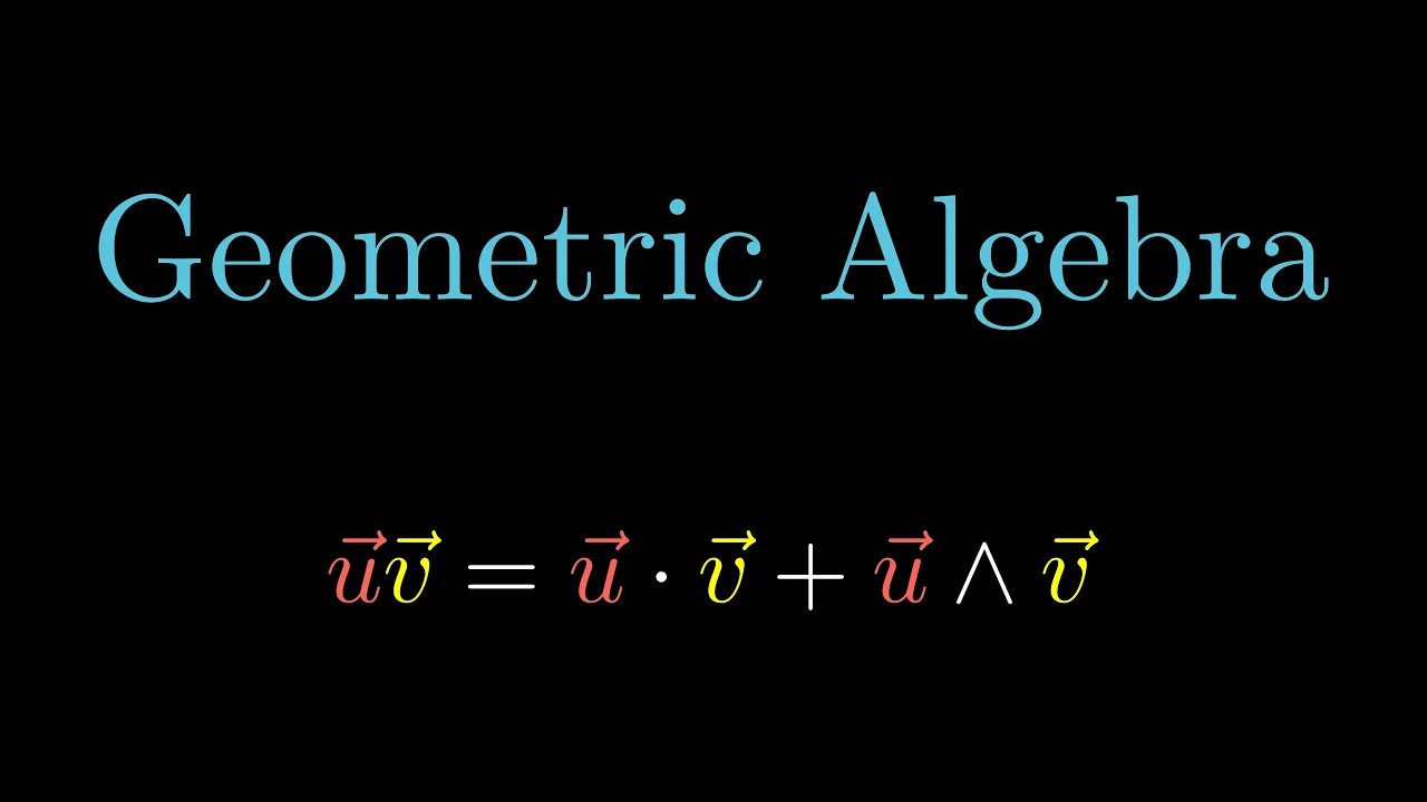
Geometric Algebra extends an n-dimensional vector space equipped with a scalar product into a 2^n-dimensional multivector system, containing scalars (grade 0), vectors (grade 1), bivectors (grade 2), trivectors (grade 3), and pseudoscalars (grade n), where the geometric product serves as the central operation that generates all multivector objects from the original vector space.
Geometric Algebra Tutorial: Vectors to Multivectors (Part 1)
Added:Fundamental linear algebra concepts, including vector spaces, basis vectors, and linear span.
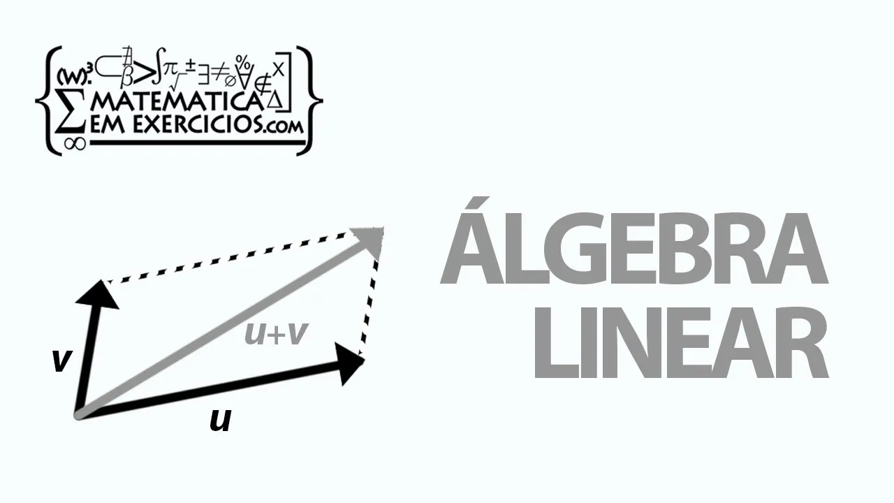
The definition and geometric interpretation of the standard dot product (inner product), including projections.
Basic notions of Euclidean geometry, specifically how distance, angles, and orthogonality are calculated in R^n.
An introductory understanding of algebraic structures, such as fields and coordinate systems.
The definition and algebraic rules of the geometric product, which unifies the inner and outer (wedge) products.
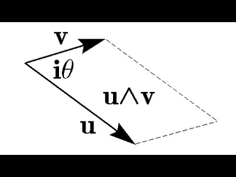
The construction and visualization of bivectors and trivectors as directed areas and volumes.
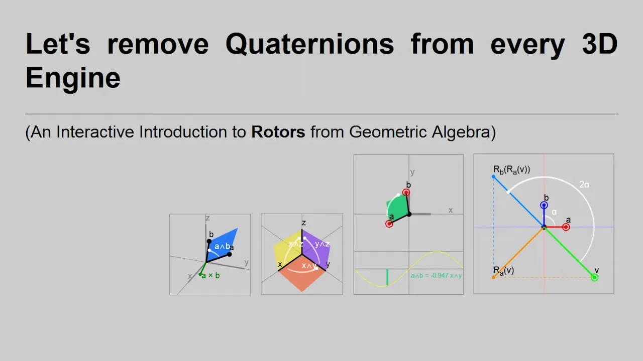
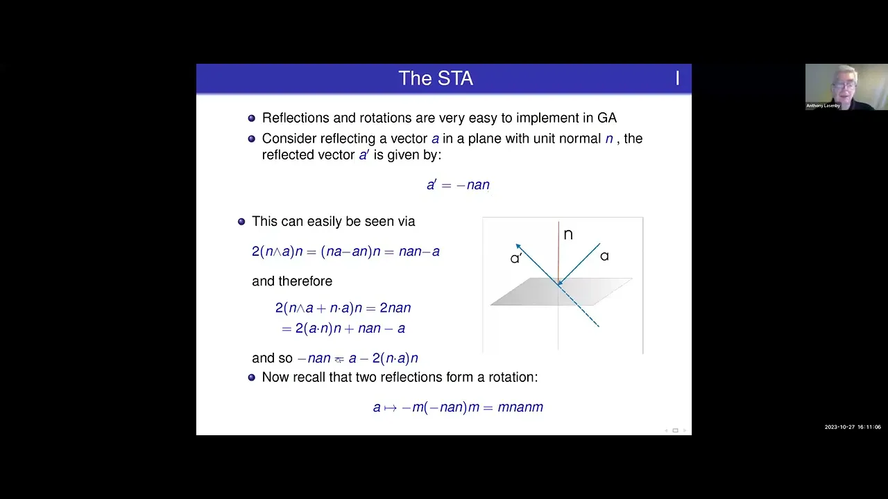
How to represent reflections and rotations elegantly using rotors in geometric algebra without coordinate systems.
Applications of geometric algebra in physics (e.g., electromagnetism via spacetime algebra) and computer science (e.g., conformal geometric algebra for computer graphics).
19.9K views527likes8:02Original Release: 2016-09-02
Welcome to this foundational video in our Geometric Algebra tutorial series. Our aim here is to demonstrate how a vector space, given a scalar product, can be extended into a multivector system called the geometric algebra of that vector space. Since this is in video format rather than a live lecture, I will proceed rapidly, assuming that the viewer will use the pause button or rewatch sections if needed. Due to size considerations this video "From Vectors to Multivectors" will be split into three parts. Though this series is designed for viewers already familiar with classic vector algebra, Part 1 will provide a rapid review of some of the basic linear algebra concepts we'll use in our geometric algebra construction. In Part 2 we'll introduce the geometric product, which is the central product of geometric algebra, allowing us to go beyond vectors and generate the remaining objects in our multivector system. In Part 3 we'll wrap up our construction and take a quick look at some of the most important examples, like G(3) (the geometric algebra of standard three-dimensional Euclidean space), seeing complex numbers and quaternions as geometric algebras (and sub algebras of G(3)), and we'll close by briefly considering the geometric algebra of spacetime. Future tutorial videos will explore these topics in greater depth, extend calculus concepts to multivector settings, and discuss alternate ways of interpreting our multivector objects for non-metric applications like projective geometry and so on. See the video description below for more information on this and other videos, and links to recommended geometric algebra resources. So...let's get started!
We begin with an n-dimensional real vector space equipped with a scalar product. Now most of you are perhaps more familiar with this dot product notation from standard vector algebra, but I'm using this angle bracket notation for now, and saving the dot product symbol for an inner product we'll define shortly. Don't worry, this is only temporary, because we'll quickly find that inner product to be equivalent to the scalar product we began with. On the other hand, the outer product that we define at the same time will be something quite different; but I'm getting ahead of myself here. For now, what we have is a finite dimensional vector space with the scalar product.
The vector space axioms allow us to add any two vectors, and to multiply a vector by a scalar in a natural way, and by natural I mean that it yields the results you'd expect. Like for instance, multiplying a vector by 3 is the same as adding that vector to itself 3 times, 0 times a vector is the zero vector, -1 times a vector is the additive inverse of that vector, and so on. But how do we multiply two vectors? The scalar product on our vector space provides our first answer to this question, and we'll see that it brings along some very useful geometric information, though a more complete answer is forthcoming. And when we introduce the geometric product, it will explode our vector space into a multivector system powerful enough to merit the named geometric algebra! We'll get there soon. But first let's do a quick review of the geometry that comes with having a scalar product. Recall that a scalar product is bilinear, symmetric, and positive definite; though it's common to relax that third condition a bit and simply require the product to be non-degenerate, especially when we want to explore the geometric algebra of say a Lorentzian manifold like spacetime. By the way, I should point out that the common practice of writing little arrows above the letters or using bold font for vectors is not a convention carried over in geometric algebra. Anyway for now let's move forward under the assumption our space is positive definite. In this case the scalar product defines notions of length and angle. We want the product of a vector with itself to be the square of its length, so we define the length of a vector like this. If you don't have the positive definite property, make sure to insert absolute value bars around the scalar product under the radix.
For the angle between two vectors, recall that the Cauchy-Schwarz inequality tells us that the absolute value of the scalar product of two vectors is bound above by the product of the lengths of those vectors. So for any two nonzero vectors u and v, this ratio here is bound between -1 and 1, which just so happens to be the domain of the our cosine function, allowing us to define this expression here as our angle. Notice that this ratio is equal to +1 when u is a positive multiple of v, meaning that they're pointing in the same direction, which means that the angle between them is 0, which is precisely what you get from arccosine of positive 1. When they're pointing in opposite directions u is a negative multiple of v, so this ratio is -1, and arccosine of -1 equals π or 180 degrees as expected. Sidenote: the Cauchy-Schwarz inequality is not valid in spaces with mixed signature, and that's why we're focusing on positive definite spaces for the time being. Taking this as our definition for the angle between u and v gives us the familiar geometric interpretation of the scalar product. Alternatively, instead of starting with a given positive definite scalar product and showing how it defines notions of length and angle, a more synthetic approach would be to begin by assuming you have notions of vector length and relative angle (as you would measure with a ruler and a protractor) and use this result here as the definition of the scalar product. From that point of view these equations become results rather than definitions. That happens to be my preferred route when first introducing students to vectors. In any case, what we find is that the scalar product of two vectors u and v gives you the length of u times the projected length of v in the direction of u, or equivalently the length of v times the projected length of u in the direction of v. When the angle between u and v is obtuse, the projected length is in the opposite direction, resulting in a negative scalar product. These considerations motivate the following definitions of parallel and orthogonal vectors. We say two nonzero vectors are parallel (or collinear) if one is a scalar multiple of the other, so parallel vectors could be pointing in the same direction or in opposite directions. And we say two vectors are orthogonal (or perpendicular) if their scalar product is zero. So our scalar product is positive for acute angles, zero for right angles, and negative for obtuse angles. But notice that these definitions do not involve θ, so I can still talk about vectors being parallel or orthogonal even after we drop the positive definite requirement on the scalar product.
Now here's where I'll assume some basic linear algebra knowledge from the viewer, starting with the result that our n-dimensional vector space V is isomorphic to R^n, which we sometimes write as R^{n,0} to emphasize that the scalar product is positive definite. With our scalar product we can easily construct (via the Gram-Schmidt process) an orthonormal basis for our vector space. The "ortho" part of orthonormal means every pair of distinct basis elements are orthogonal, while the "normal" part means that they all have length one. Sidenote: in a mixed signature space V is isomorphic to R^{p,q}, so our orthonormal basis will have p basis vectors that square to +1, and q basis vectors that square to -1. By Sylvester's law of inertia, p and q are basis independent, meaning that for any fixed finite dimensional vector space with a non-degenerate scalar product, the values of p and q won't change if you change your basis.
And if we allowed a degenerate scalar product, the index of nullity would be a fixed value as well, but let's not get into degenerate spaces here. In Part 2 of this tutorial, we'll see how to go from our n-dimensional vector space V to its 2^n-dimensional geometric algebra G(V).
We'll see that the geometric algebra of V contains within it scalars (which are the grade 0 objects), vectors (which are the grade 1 objects), bivectors (which are grade 2), trivectors (which are grade 3), and so on, all the way up to n-vectors (the highest grade objects in the space) which are also called pseudoscalars. General elements of geometric algebra (called multivectors) are formal sums of graded elements (called K vectors) which will be introduced in the next video. All this will arise naturally, simply by the introduction of the geometric product. So please come and join me in Part 2 of this tutorial From Vectors to Multivectors!
Up Next
36:26
Geometric Algebra: Rotors and Quaternions Explained
@Math_oma
17.1K views•2018-06-19
51:00
Conformal Geometric Algebra Explained: Lines, Spheres & Inverse Kinematics
@bivector
1.5K views•2024-09-05

10:44
Fourier Series Introduction: The Big Idea Explained
@DrTrefor
387K views•2021-05-03

6:00
The Mathematical Impossibility of Accurate World Maps
@Vox
23.3M views•2016-12-02
Related Study Plans & Knowledge Roadmaps
Structured learning paths in Mathematics
mathematics
Tensor Calculus: Vectors to Riemann Curvature
01Mathematical Foundations: Linear Algebra & Calculus
02Covectors, Dual Spaces, and Tensor Basics
03The Metric Tensor and Index Gymnastics
+ 2 more learning modules
40h5 modules
Explore Roadmap
mathematics
Gödel's Incompleteness: Logic, Proofs & Limits
01Introduction to Formal Systems & Hilbert's Dream
02Set Theory, Cardinality, and Cantor's Diagonal Argument
03Arithmetization and Gödel Numbering
+ 2 more learning modules
14h5 modules
Explore Roadmap
mathematics
Galois Theory: Fields, Groups & Solvability
01Foundations of Abstract Algebra: Groups & Fields
02Polynomials & Field Extensions
03Splitting Fields & Symmetries
+ 2 more learning modules
24h5 modules
Explore Roadmap
mathematics
Non-Euclidean Geometry: Models & Geodesics
01Euclid's Fifth Postulate and the Birth of New Geometries
02Hyperbolic Space and the Poincaré Disk Model
03Geodesics: Defining Straight Lines in Curved Spaces
+ 2 more learning modules
15h5 modules
Explore Roadmap