







![EE361 [S21] Stochastic Signals and Probability Pt. 2 - Signals and Systems II](https://i.ytimg.com/vi/6XTvBk_o7kA/maxresdefault.jpg)




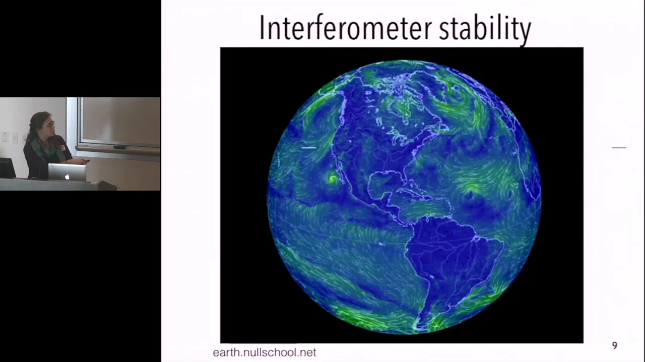




In gravitational wave detection, Gaussian noise is characterized by a probability distribution where values farther from the mean are exponentially less likely, with the standard deviation (sigma) controlling this decay rate. When analyzing detector data, the noise can be modeled as a multivariate normal distribution in the time domain, which simplifies dramatically in the Fourier domain due to stationarity—where the correlation between noise components depends only on their time separation, not their absolute positions. This allows the power spectral density (PSD) to fully describe the noise, making the Fourier-domain covariance matrix diagonal. The optimal signal-to-noise ratio (SNR) is defined as the norm of the signal vector in this noise-weighted inner product space, enabling efficient detection through matched filtering. For multiple detectors, the network SNR combines individual detector SNRs in quadrature, leveraging the statistical independence of noise across different locations to improve detection sensitivity.
Gravitational Wave Data Analysis: Gaussian Noise, PSDs, and SNR
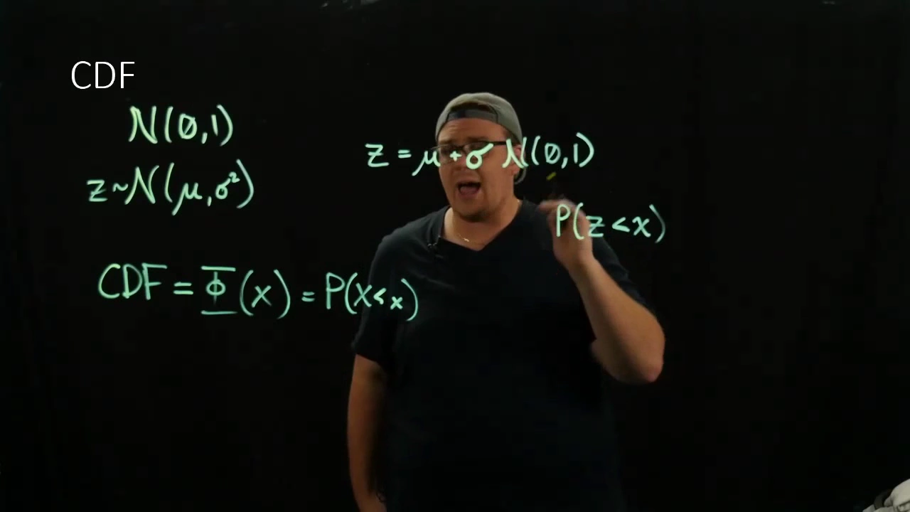
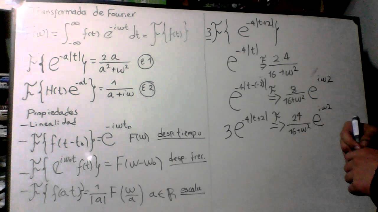
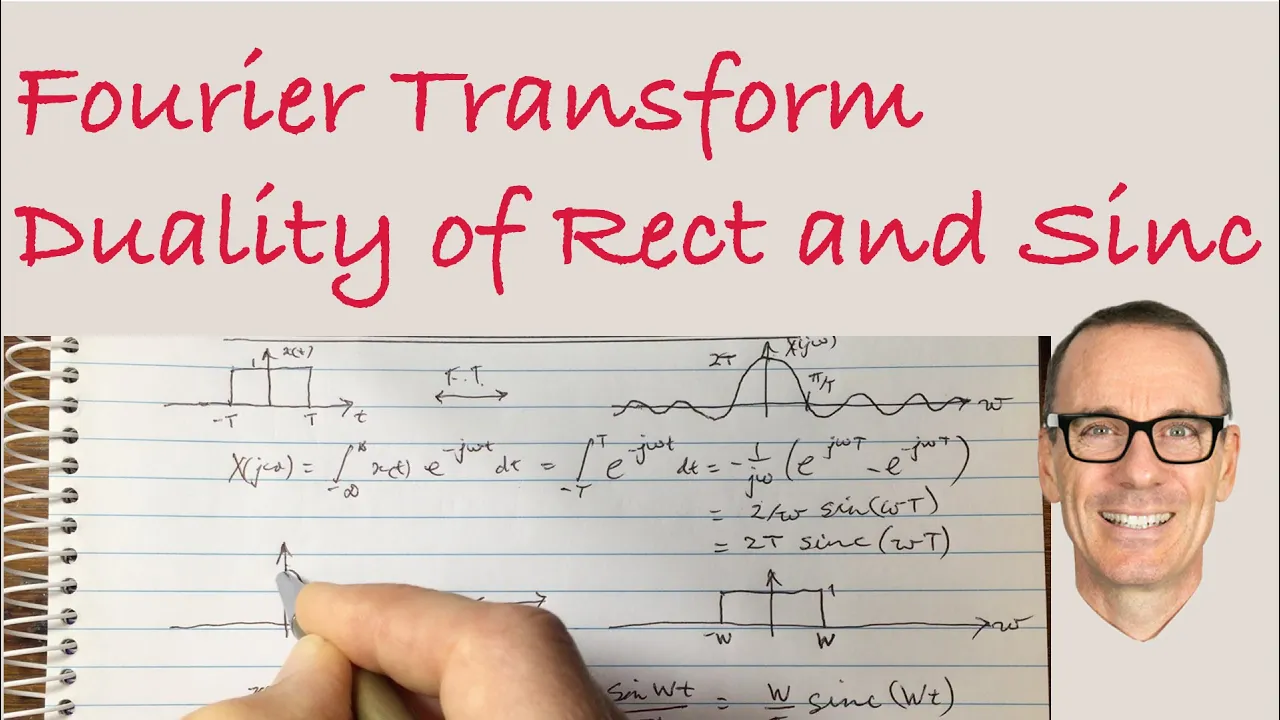
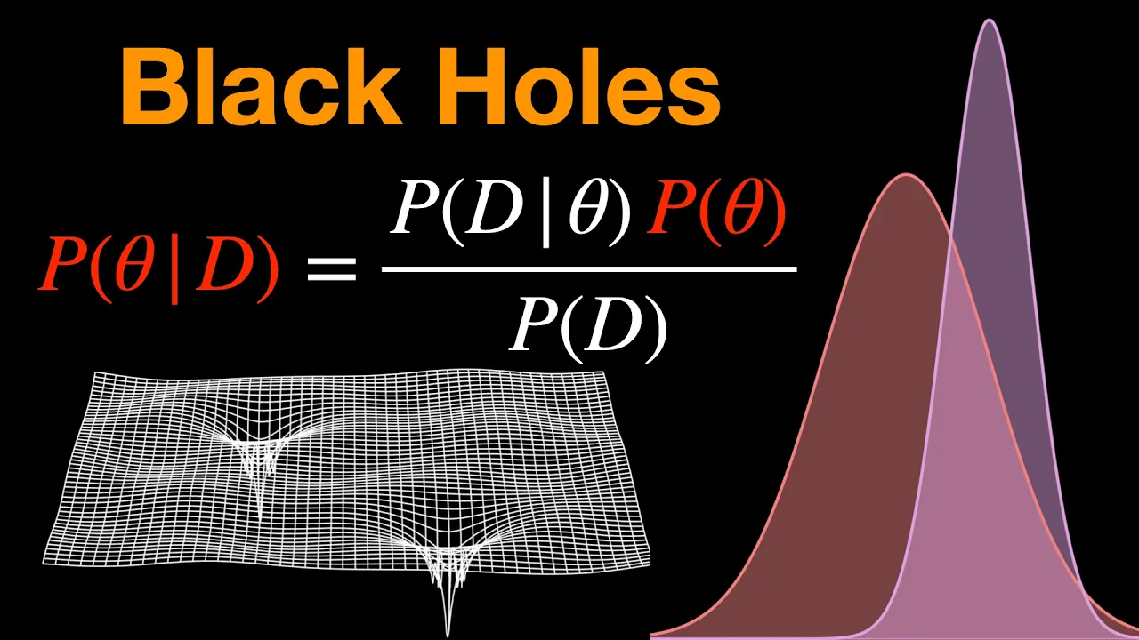
Added:hello all right it's six minutes past nine so we might as well get started okay so yesterday I spent a lot of time talking about all the properties of the noise and all the ways in which it's complicated and imperfect and by at the end I started focusing on the idealized case in which we can assume that the noise is nicely behaved and Gaussian and has these nice statistical properties which is what we will in many under many circumstances assume because we trust the whole infrastructure that we have in place to Vito characterize the noise and make sure that the parts that we're actually analyzing actually conform to these assumptions and we can quantify that degree so today I decided to step back a little bit and make sure that we're all on the same page regarding what Gaussian noise is and what properties he has that we will be extremely important for what we do later so I'll slow down and and go over some of the steps here a little bit more before we actually get to to the signals if we do in the end I understand yesterday maybe you had a little session on trying to get the data online did anyone actually go to the website and do stuff or no do you guys okay so maybe before we actually get to the signals I'll just show you how to access the data that we make public and how to I'll point you to some of the tutorials so you can start already putting in practice some of it the things that we've been talking about you really have a lot of the basics for what you need to manipulate our data so so have an interlude before we actually go to the signals you'll notice that this is a third lecture and I still haven't gotten to the signals right so when you perhaps if you're not in the field you think that beta analysis is all or what we do in Lagos all about the signals but really it is about understanding our instrument and understanding the properties of the day then only once you're an expert in that and you know what you're doing only then you get to go to do physics or as astronomy with your data so this should be a moral lesson if you wish anyways so there was a question yesterday about the you asked me about what is this stuff up here and I asked my friends at Caltech and they're like it's calibration lines that were moved there used to be a 33 Hertz and now they moved them back here and so that's the answer this it's no mystery noise that's why they're in both Hanford and Livingston detectors maybe no one cared but I wanted to to clarify that all right I don't have in my head the latest you know basin exchange and so we have experts in the group that really keep tabs on all these things and they are documented but I forgot all right well and you see that very good as things differently right so okay so this is our basic our starting point for all we're doing today and we were doing yesterday so we have the data we have that may have some signal but mainly dominated by noise and today we will be focusing again on the case in which we can assume that the noise is ass nice as we can take it to be again to make sure that we are all on the same page right noise is by definition a random process it's a process that creates random numbers okay a random variable is said to be Gaussian if it follows this probability distribution okay it's just a probability distribution that tells you values that are farther away from some mean are less likely exponentially with some scale set by the standard deviation or Sigma or the variance Sigma squared okay you should have seen this in like kindergarten how do we interpret this well you can think of this as what's the probability if you're drawing if you have a black box on you just it's spitting out numbers what's the probability that you get some number given the the process is defined by this function that's when we are thinking about it it's not the best way to think about it the best way to think about it would be if you are in a casino and they are Tibet what's the next number going to be you should be placing your probability sure you're betting odds you should put more money on values that are closer to mu and less money would've Alice are far away and this is what we call the betting odds or Bayesian interpretation of probability which is important to keep in mind there's a slight distinction in saying well what's the distribution of things as they're actually happening versus what's my belief on what's going to happen okay so this may come back to bite us later that's why okay so a Gaussian Gaussian distribution for normal distribution or Gaussian for a single random variable with no mean and standard unit standard deviation looks like this again it's just saying that the farther away you are from the mean the less likely you are to the less belief you should usually assign to this to getting a value of x that is farther away from the mean this is the probability density this distribution the probability density function PDF so we'll use this over and over again in in our work okay so when we have a noise series so let's say you've taken a bunch of LIGO data you have observed for some time T and it's sampled at 16 kilohertz you have a bunch of data points well the correct way to think about that if there's no signal there and it's just Gaussian noise is to say that each of the each of the data points corresponds to a given random variable right so a random process is actually a collection of random variables so you should be thinking about each data point some unknown random variable and you'll assign your belief to what you think that each of them what what's the value that each of these ends should take right so think of each of them as if their own random variable they will they won't be uncorrelated variables right because if you know something about and no and zero you may know something about n1 because you know for example that LIGO has some high frequency noise that will correlate the two two data points taken one after another in some particular way but you are still different random variables just no independent ones if the noise is Gaussian this set of random variables will be described by a multivariate normal probability so it's just a generalization of the probability density function I showed you earlier except it will have instead of one dimension it will have n dimensions where n is a number of data points in your set okay so you have n variables each of them is distributed in according to some probability density function like this and then so the whole thing is described by the the joint probability function which is a multivariate normal so the way we write that down is a generalization of what the exponential expression that I showed you earlier so you see e to the minus 1/2 and I should say this is proportional to because there's some normalization here that I don't care about right the whole point is that a PDF should always integrate to one right because once you can see all the options the outcome should be a hundred percent so so you can normalize the probability function accordingly but we don't usually care that much about the normalization anyway so if you have n random variables then the generic gaussian multivariate likelihood will look like this inner product between the noise or the data vector weighted by this covariance matrix which is a generalization of the variance that we had in one dimension so if you have a process in two dimensions so you just have two data points you can use to visualize it this plot from Wikipedia okay and so you have two variables along the two axis and they're each described by some Gaussian probability function but the two are not uncorrelated right there's some there's some information here right if you know that X the this Y variable is towards four then you know the x1 X variable is also likely to be higher and so you see there's some correlation in this direction for example does that make sense that's information that gets encoded in this covariance matrix right so in the simplest case the blue and the red curves are just two Exponential's two normals and that are independent of each other and then this thing in the center is just a circle which means that you have if you know something about X you don't know anything about Y and vice versa and in that case this covariance matrix would just be zeros everywhere except along the diagonals and the diagonals are just their variances of each of the two independent processes right so again if you just have one dimension then you just get the covariance it's just Sigma squared right it's this all making sense to you let me know if you want I get speed up or slow down according to your to your needs in this case where you just have two dimensions you can parameterize the off-diagonal terms in terms of well this the individual standard deviations and some correlation parameter Rho that can go be to negative one and one which tells you that if Rho 0 then the variables are totally uncorrelated if it's absolute values one they are maximally correlated so basically they're the same ok whatever it is CIJ has always has to be diagonal right because it's symmetric right if I know something about if something about X implies something about why the other one is the opposite relation so which is also true so even in higher dimensions this will be a symmetric matrix ok everyone with me math in the morning might not be the best thing for you but it's good for the soul so just work through it they stay up you can go have some coffee we'll take it right all right so the next step is just ok so this was valid just in general for any Gaussian process and that that includes processes that are evolving in time but we can make the further assumption in our case when we're looking at short stretches of data that the properties of the noise are not changing was the meat wasn't mean short well the noise is created by the instrument and its environment right so it can be the thermo thermo the thermal motion of the surface of the mirrors and the coatings it's just creating some fluctuation in the profile of the light or it can be some shaking in the violin modes or whatever it is some physical process and so that noise will be intrinsically related to the properties of the instrument at any given time and as long as you're looking at times that are short too with respect to the scale over which the instrument may change right let's say you know the alignment of the mirror the optics may change over hours or in in slight my new ways and may alter the specific kind of noise so you get in the instrument or there might something might happen there might be an earthquake somewhere half a half across the world and then it shakes everything up and the whole instruments like a new instrument all of a sudden as soon as you're not in that situation if you're looking at say a few hundred milliseconds or whatever where you can be confident that your instrument stable and the environment is stable then it's reasonable to assume that the statistical properties of the noise are not changing just because the physics of the instrument are not changing okay so in that case that means that the correlations between so remember I have a series of random variables and each correspond to a point in time because each of them is a data point that I've taken then the correlations between those points if the process is stationary by definition only means by the definition means that it only depends on the distance in time between the points not where they where they're located right so if I let's say I take a bunch of data points these are my ends and zero okay if the process is stationary the correlation between two points let's say in general I and J will depend on this on the distance between them in time right this axis this time but it won't depend on where I place this interval right as long as the distance it's the same the correlation should be of the same magnitude right there's a translation symmetry in space in time that make sense so if I look at shorter shorter intervals then yes the correlation will be different because points that are closer together are correlated by higher frequency noise and points are farther away are correlated by lower frequency noise but it doesn't matter where in the in the data stream and looking at so that's what this expression is saying is that the correlation between two points index by I and J just depends on the on the distance between them in time but you can write them in terms of the distance and indices right this is just the time J and the time the variances are yes because it's zero lag yes it's just yeah basically what you get the formula you get for a matrix like this is so well if you had more more rows you get something that's like cyclic so it's the the the they come the elements start it's like rotating around so you would let's say we have three it's easier to see in there CIJ and I have Sigma X square well let's go which that you see okay C 1 1 C then this component will be that same thing and this will be C 1 1 C 1 2 and it will cycle around because it should only depend on the difference and it has to be symmetric and this has a special name called top let's kind of matrix if you care that's right I think it's I never know is it oh let's put something like that anyway so it clearly has some nice symmetry properties Cement some nice symmetries that we it's what we will be able to exploit but the the symmetry becomes manifest when you actually switch to the four-year domain and you take a Fourier transform of this object essentially you take a Fourier transform of so this is a covariance matrix we call this the autocorrelation function it doesn't matter one of the rows you take the Fourier transform of that you will find that that corresponds to a power spectral density and if you look at the of the statistical distribution of the Fourier domain noise then it will be diagonal so if I instead switch to if I Fourier transform my noise data and I look at what the what's the correlation matrix for the for the amplitudes in the Fourier domain right so that's a tilde here for Fourier domain then you'll find that for this for the same kind of the same noise in the Fourier domain this correlation covariance matrix would just be diagonal and you'll have the PSD in the in the diagonal and everything else will be 0 so it's just like a change of basis right you if you found it sort of happens that for this kind of process you changed the basis to describe what's going on any diagonal Isis in the Fourier basis and you can just it takes a very simple form so that's the reason why basically all of the analysis in live are carried out in the Fourier domain because it's the noise stationary has this nice property that it simplifies in the frequency domain ok so let's unpack this a little bit or a lot ok this is a way of defining what the power spectral density is which as we will see it's the square of the amplitude spectral density that I discussed last time okay so this is math so this is just a bunch of ways of writing the same exact thing in different ways that illuminate different aspects of it so let's just maybe let's do you dare do you approve okay let's see we can show that the PSD is actually so we can show that this is true and that the correlation between that's the correlation between the Fourier amplitudes so if we turn our Fourier transform I by noise n that's it till there right and then I have a function of frequency instead of time and then I look at this the square brackets mean expectation value so what's the average that you should expect for this product of the two of these two quantities you take the you take the conjugate because now it's complex and you want something real okay so and then you find this is the same the same definition as for the C before right except now in the Fourier domain and then you find that that there's a function that exists such that the correlation is one-half that function and then it's diagonal so only you only get correlations for the same frequency okay so let's show this okay so first we have by definition the Corey I'm going to define the correlation between the noise sometimes I put the end to remind us that it's the noise but then I forget whenever the correlation between the noise at frequency one and at some frequency and some F prime and other frequency F prime its I defined that to be right the expectation value which is what this angle brackets denote of just the product of the amplitude of the noise at the first frequency times the amplitude of the noise at the second frequency okay then I want to show that this is a simple it there's no correlation unless the frequencies are the same essentially that's what the first line is trying to say and how large the correlation is is said by this function S which is called the PSD okay so these are just Fourier transforms of the noise so I can I can insert the integrals this will be fast D DT can you see this by the way because if I'm standing here for 30 minutes in the upper if you can't see there's no all right so let's expand this so this is just the first n tilde right and there's the frequency F here and the same thing for the second one except now let's use another dummy time called t prime e to the 2 pi I might have the minus signs wrong oh no that's fine there's no minus sign here because I had a complex conjugate okay but I do have a minus sign here that's just by convention of the Fourier transform T prime okay just explicitly what whether Fourier transform is now I can define a variable called tau which will just be the difference between the two times okay it's just a change of variables and in that case I can make this look like an into a double integral over of T and then this is going to be n of T plus tau right so I'm gonna incorporate in with the noise at a some lag towel afterwards right and so then I won the expectation value of that and then you have e to negative 2 pi I tau eat right so now I have an integral over over the overall time and an integral over the lag between the two points Tao okay the integral over T so I can carry out the integral over T and then just get a delta function between the frequencies oh because there's an assumption here remember that it's stationary if the noise is stationary as I argued earlier this shouldn't depend on the actual time T right whatever time it only depends on the lag between the two points and this is the same thing I was calling see right is the quarry is the correlation I was going at CIJ but in here where we're in the continuous case so let's go see T and T plus tau and by definition of stationary it just means that this is just a function of tau can you see this I guess this is bad practice should I use a different calling alright this is not part of the main equation it's just a reference to this so this thing doesn't depend on T even though it has T in it apparently because we say it doesn't by assumption of stationarity so then we can just carry out the integral of this exponent exponential and it's just a delta function between the two the two EPs and then then you just left with let's call it C I don't know if anyone actually sometimes this is called R okay so you already see that we've shown that stationarity means that the correlation between the noise at two different frequencies will not only be nonzero if the frequency is the same so this this matrix will be diagonal it means that the independent frequency components of the noise are the different components of the noise in the frequency domain are independent because of this delta function and then you have this term and that's where that Vener kitchner whatever theorem says that you can define a nice function called the PSD that will have this value and you can write this as F minus F prime okay all right so essentially it's just the fact that if you assume stationarity then the correlation between the noise and the time domain doesn't depend on tau and so this tau at the t4 falls out you can you get a delta function here and that tells you that this thing should be diagonal yeah the way that the data taking process is done if you're done sample or whatever you're supposed to have filtered away anything outside the band so that it doesn't leak back down but yeah I mean I've done here in the ideal case where you know this integral sir from infinity to infinity in reality there's a well that's my next line in reality there's a band limited version of this in which you only have resolution between some mean and if Max and between some and I'll show that next but anyway so you can take this as the definition of the PSD band then if you do that you find that you can write it because of how we so the angle brackets are the expectation value right that means what's the average value you should expect you can always estimate that by just doing a simple time average right I look at this this random variable X for a long time I integrate and I divide by the time I looked at this is just does everyone see how this is an average over time okay so this is an assumption called there go disa T which means an average over ensembles is the same as average in time but it doesn't matter so you can use that to rewrite this function SN the PSD and you can write it as this and you'll see that this is just well or just from here you see that this is just the expectation value of the square amplitude of the fourier of the Fourier amplitude of the noise right so this is just the Fourier transform your noise you you get an amputee complex amplitude you take the norm and the expectation value of that over several instantiations of no system is what the PSD is yeah it breaks in different ways so we'll mention some cases but ok you can break because your perhaps you're analyzing a signal that's very long in the in the timescale of the instrument and so the the Gaussian properties are changing but that would have to be I don't think we're still in that regime yet the signals we see are at most you know yes yes you you would do the analysis in a different way you for example split it up into chunks over which you can assume it's stationary we have others other searches like searches for continuous waves that are on all the time in that case of course you can't assume this noisy stationary throughout the whole observation so we have techniques effectively what you do is just chop it up into smaller chunks over which you can estimate the properties you you add a time dependence to to this F but it's low compared to the frequency of the gravitational wave for example so that's one way that's easy to deal with right so Gaussian noise is itself changing very slowly as soon as it's changing slowly with respect to a frequency of the wave that you want you're fine it's like a stationary phase approximation then you can have stationarity break down if for example there's a glitch just as you're observing your signal this happened with the first binary neutral detection in 1708 17 right there was in one of the detectors we were seeing the signal very nice you know the Sun blue there was like this shaking for some reason just overlapping with the signal in that case it's harder right you obviously it's not stationary it's not even Gaussian so we have techniques to subtract that from the data using the fact that do you think of here and sequester detectors and so on and and clean it so that it looks as soon as possible but of course yes this is a limitation but we have ways of evaluating how close but it's not like we have to blindly assume it's stationary we can say okay how close the stationary is yeah okay so let me another other questions immediately yeah it is a power spectrum yeah same thing except in cosmology your signal is Gaussian here when talk about the noise but it's the same thing I don't think so oh yeah to us a test yeah yes sure we have we have many ways of about many markers of Gaussian a you know the the thing about Gaussian is you know very well is the there's one specific way of being Gaussian basically but there's infinite ways of deviating from Gaussian e and that's you know in cosmology if you want to say a background Gaussian or not you can't just look at one marker and say you know the kurtosis is zero so whatever it's it's Gaussian but yes we compute those things we compute many other things base factors perhaps tomorrow I can mention a few of those if you're interested by the way you should feel free to request focus if you if there's something you want me to cover so I'll make a point of mentioning some of that oh oh yeah so we also have case if I have time on the last lecture we'll say something briefly about how we search for stochastic gravitation way backgrounds in which case the signal itself has properties like this it's kind of like in cosmology so it might be interest since this is a workshop on cosmology also I'll make sure to cover that ok so any last line here so we found that the correlation of the Fourier amplitudes you can just it's just diagonal and the magnitude of it is determined by this function at PSD you can note here in the last nine that this function the PSD is just the expectation value of the square amplitudes of the of the Fourier domain of the Fourier domain amplitudes of the noise so you just take the four you take a Fourier transform of your noise you take the norm squared and then if you have several versions of this so that you can average over it you get an estimate of the PSD ideally this average you would need infinite data to estimate the PC perfectly so it's like anytime that you want an average you get an estimate of the average write it form from any real finite instantiation of data so this should ring a bell because this is basically what well it's just method was so I hope this clarifies a little bit where that came from because I sort of put it out there out of the blue right but the reason that when we are estimating that the statistical properties of our of our noise from the data that we take this this approach basically as you remember in that case we will grab the whole stretch of data let's assume it's just noise right we split it up and we take the P we take the Fourier transform we average the amplitudes over several segments of that well that's just estimating it's just estimating this right it's just taking turn to estimate the average the expectation value for this square amplitude for you is that if that makes sense do you remember what this was it was yesterday so hope your memories longer life all right now there's a point of Ricardo brought up and that came up earlier which is in reality we don't have infinite infinite resolution or infinite observation time so you have to modify or adjust these things a little bit the difference the main difference here is that when you instead of getting a delta function this integral of their time here instead of being I am assuming here it was going from negative infinity to infinity in reality we'll go from T over 2 over to t minus T over 2 to T over 2 where Big T is the observation time you're serving over so you don't get exactly a delta function here you get something that we call that we denote like this Delta sub T so I can approximate Delta function that makes sense you don't actually have infinite were you raising your hand yeah can you say it speak a bit louder sorry we're trying to estimate the properties of the noise there's no signal here yes no this is I mean you could do for the signal but the signals not a stochastic process the signal has a well-defined so all of these if you did this for the signal you'd be wrong no I mean we did for the data over a over a period of time for over which we don't expect a signal to be there it was a short CVC signal was indeed here in let's say would be in like one of these segments very short spikes if June a 14 happen here it gets averaged out mostly for the most part right so in this process it just gets washed away so this is just to estimate that the the statistical properties of the noise that dominate the data and separate that from the signal and I should say this is not the only way of the of estimating the PSD we have more complicated ways of doing so but okay so back to here the the difference is that you don't get a perfect Delta function there you should get this this approximate Delta Phi you know if you if you let in the limit that T goes to infinity this is the normal function of X okay but if it's not infinity you actually can compute this integral and it's something that if the argument goes to zero it doesn't go to infinity it goes to T okay doesn't make sense so as X goes to zero this this delta T function goes to the Big T okay so you can see here that as the frequencies close arbitrarily close to each other this term doesn't go to one it goes to T and this is a tea that comes in and it's what shows up if well if you so this I'm still in the continuum limit if I take discrete samples and this becomes C till the I J right between frequency high frequency J and this is Fi and then T is just one over remember that the frequency resolution is 1 over T so that's where that comes in here okay so okay so after all this and we convince ourselves that the correlation the covariance matrix of the Fourier domain noise is diagonal and it's given by the PSD go back to why were we doing this in the first place right and it was just because the probability that we wanted to write the probability of having some noise given some statistical properties and if I Fourier transform this expression what I will get is that I can write it in terms of the probability of my noise if I assume it's Gaussian with a PSD s it's just going to be the sum over so it's n I and I because it's diagonal right the Delta function and then oh yeah so divided by the PSD and then you get this Delta F for a frequency resolution that comes from from this thing this is makes sense to you it's it's I want to estimate the probability of getting some Gaussian noise right and I can write that in the Fourier domains in terms of the Fourier components of that noise and weighted by the PSD this as you see it's just an inner product between the the noise vector with itself right so we can generalize this this this term here and define the inner product between X some some data some time series or frequency series x and y as four times the real part of this of this integral which is just as you see it's just a regular inner product except we have some measure defined by the power spectral density of the noise and this it should look just like a Gaussian to you essentially where this takes a role of the variance right and this is that it's the it's like the distance between x and y okay let's see that but the point is that you're waiting this this term by the sensitivity of the instrument as I mentioned yesterday so frequencies for which we're more sensitive have a lower PhDs and so this number is larger and for frequencies over there's a lot of noise and this is a large function we don't count that that much in the inner product okay so we can write the likelihood that's the inner product of the noise itself okay and so this is very nice in the Fourier domain okay questions are this basic mathematical gymnastics yeah so let's look at that now so imagine there's actually a signal in the noise now let's put back H in there whatever that H is it's some function of T or frequency it's H of T right and it happens if it's a compact binary signals a short signal whatever but now your data are H plus n not just n anymore so what's the probability of getting some given data D that has a signal in it H that I know exactly what it would look like well just rewrite this expression and you just get that the residual between D and H so you take your data subtract that the template that you expect and you get the difference between it we call the residual that should just be distributed like the noise right do you see this N equals H all right and we know by assumption that the noise is Gaussian and so on we'll just have the all the statistical properties that we work so hard to define over the last since 9 a.m. ok so then the probability of getting some set of data D that has a signal H in Gaussian noise that has a power spectral density S will just be this inner product as it was for the noise only K so they know some of the cases just where H is 0 then then N equals D and then you have the same expression you have before do you see this I'm just subtracting yes so in this case I'm saying I want to know what the probability of the data containing a specific age that I have a model for right so I know I want some specific H of T that it's let's it's my target right so I want to know H of T will be something whatever that I can predict as a function of time it's that specific age so and I have some data that's noisy and so how I can how what's the probability of the data containing that signal age and having Gaussian noise s okay they likelihood rather it's this quantity P of the data given this assumption and it will be this we call this kind of probability where we have the data conditional on some model of the signal and some understanding of the noise the likelihood and it's in red and bold and underlined because it's a very important term right that comes over and over again and we'll say the likelihood like I mean it's it's the bread and butter of what we do okay and we use some curly L symbol to denote that likelihood but it just stands for this it's just a shorthand for for this probability yes there's no noise part of the signal there's no part of the data okay so but yes it depends on the on the noise right the noise is coming in so there's noise in D D is H plus n this is noise and s is a property of the noise it's the thing that describes the correlation of the noise in Fourier domain this is fixed by the instrument right the instrument tells you how nice it is at different frequencies these are it's like the plot I showed the very first part I showed today and this is just whatever signal you're looking for I want to if in the ideal case yes except if the data are taking very far away in a long time apart then this s will be a different thing for so for different events you'll have different s just because the instrument has changed in between that make sense so if the if the instrument actually didn't change at all and was perfect then yes it would they s would be the same for everything but over as I mention over longer periods of time the instrument is changing so this function will change so you have to estimate this every time that you do basically well the simplest way is let's say I think there's a signal this time t0 I'm gonna I know the signal short it's only whatever 200 milliseconds I'll go one second before that and now look at the noise there I now assume that over a period of many seconds the noise doesn't change you can still do that except I mean as long as as long as the scales you can go minutes before or like whatever you need in general we can evaluate whether the no except in changing or not but it's a good question and the answer is we don't do it in the way that I explained before we don't use this Welsh averaging that requires having pure fewer noise only data to estimate it we actually fit for both the signal and the PhD at the same time simultaneously so we have a complex machinery to actually estimate both H and s at the same time using the data only that has the signal and the noise without needing to go off source which is what we call that I will discuss how we do it for several waveforms tomorrow for now we I need you to understand what happens when you know exactly what waveform you want so that part of parameter estimation will be allowing these things to change oh wow all right one two three yes look it up I don't remember how but yes yes it there there's some information content that you can extract of your sip for you from your signal and then it's determined by yes I don't remember but we do use those quantities every now and then in our papers you see you extracted so many bits of information from the data and it's computed using that but s it's not entropy itself yeah yes tomorrow we're doing that but yes so the obvious next step right I mean but first imagine you know exactly what it's like then we'll have actually a whole set of different possibilities and we'll sort of iterate over them we don't do that exactly that way so speak yeah so for a signal for for a if we're searching for a compact binary signal a short signal then and you have a lot of a very loud stochastic gravitation way background that will act as noise to you in the search for the compact binary signal in much the same way as instrumental noise does so there's no difference whether the noise is coming from the instrument or if it's just because there's actual gravitational wave I mean it's actually the if it's actually worse if the noise was dominated by the stochastic background it's even worse because it shows up in all the detectors at the same time whereas this s is if it's instrumental it's just said before each detector and it allows us to see the signal better but so if you're doesn't make sense so that kind of signal would act as noise if you're looking for shorter signals and this is what happens with Lisa for example Lisa the laser interferometer space antenna that supposed to fly in 2034 will have so will be so sensitive that it will have this constant background stochastic background from white dwarfs that it's gravitational waves but they essentially are a source of noise to all other analyses and so you have to dig out signals from the the noise and gravitational waves but it acts in much the same way as any other noise I mean the whole detection technique for stochastic backgrounds will rely on the correlations of the fact that we expect instrumental and environmental noise to be uncorrelated for the most part but correlated noise in all detectors would be associated to a gravitational wave so that's the key to try to distinguish a gravitational wave noise from some more boring noise it will be the correlations yes of course and it's it's one of the things I mean to cover in the last lecture so this so this formulation actually applies in general to any signal you want to look for but the specific way in which you implement it changes a little bit if you're searching for compact binaries which is what I will focus on right after this or these longer signals like and you will rely more in some cases coherence or other things but all of this this formulas in applies oh but I've come back to otherwise a piece for now all right good so one concept I want to introduce is whitening so if you look at at this inner product the way we defined it well I had written it XY over SF but you can write it as you can assign you can take the square root and assign one square root to one of them and one square to the other okay I just split this into two by taking the square root and so you see that you have these quantities that are the Fourier transform data series weighted by the square root of the PSD each of these two factors the square root of the PSD is the amplitude spectral density which I mentioned before and so you find that for Gaussian noise if you just do this then the quantity n tilde over s to the half power will have unit variance so you're basically taking noise that has a power spectral density this is invisible that's like this like in like on right there's a calibration line that I forgot the 60 Hertz line whatever and so you have frequency here and then you have some noise that is distributed according to this right so if you took the Fourier transform of the noise it would roughly follow this curve okay then if you divide by the PSD you go from that to something that's flat right so this is let's say these are n this is I just flattened out the power so I've divided by the PSD and so then the distribution of power in the of the noise in different frequencies will be the same because I'm dividing by the trend so whitening you can think of us a way of flattening the PSD it's called whitening because then all the frequencies have the same power equal contributions from all frequencies that's what white light is right equal power across frequencies another way of saying this it's the equivalent statement is that it D correlates the noise so if I then take an inverse Fourier transform of this then I'll just get Gaussian noise that is uncorrelated because there's because all frequencies have the same at the same power then the covariance matrix will be diagonal okay oh so you can do this to the actual data right and so you can grab the data you can Fourier transform it you can divide by the PSD so you you down weight frequencies are very noisy and you elevate frequencies that are that we are more sensitive finger are very noisy frequencies that were more sensitive to and then what you get is that anything that stands out of of just the noise will immediately pop out right and so in this cave of 59 14 you see here you mainly just have at all frequencies it looks the same because we have widened it whereas remember that yellow spectrum I showed you before it was very different across frequencies now we've divided that away so their lines are gone they don't appear anymore and this is so if you just plotted this it would just follow an a Gaussian distribution and it's it's true until you get something that it's no longer just Gaussian noise and it's clear that it's standing away from the it's not described by this Gaussian distribution and it shows up very very clearly here and we didn't necessarily have to filter or or do anything manually to see this by eye you just divide by you just divide away the noise and the signal pops out and it's very pretty like that anyways they the it's useful to think of whitening because we can define this quantity right so we'll take the difference between the data we subtract that signal from the data they said that's a residual and we'll divide by the PSD with this extra T here which is it's just coming from from that imperfect of function but it doesn't matter and this is just a widened residual right I took the residual and I divided by the P by the ASD right then the this quantity will actually have a 0 mean unit variance distribution so this is we've turned our problem into a problem of a Gaussian again a simple Gaussian of uncorrelated we then correlated components so that's what's going on here and it's useful to think of if the data are actually what you assume them to be so if you assume that the data is Gaussian noise plus the signal that you expected H when you subtract H from the data and you whiten it what you get must just follow a Gaussian distribution if that's not true then your assumptions are wrong something since you're the puzzled anyways yeah well first let's assume that the data are not that the instrument is not changing let's say over a day it stays pretty much the same I can go and look at some arbitrary time where I know there's the recent a signal and I can estimate what s is then I a signal comes by at a later time but I know that the properties of the noise haven't changed so I can use my estimator of the PSD from an off source we call it off source region so we go to a time where there's no signal to estimated PC but this is related to a question as earlier so that's the simplest case right in reality you can simultaneously estimate the signal and the noise from a given search of data that has both we using more complicated techniques but you don't really need to yes we release the data we release the templates mostly in some cases but we release the s which you could also compute from the data yourself but there are many ways in which you can st you know you don't have estimates of s so we release the one that we used so you should be able to reproduce exactly so you might get a different result if you estimate your PC differently and you know then we will get different results but yeah so we make s explicitly available I think in all cases this it's just indexing the different data points so here I've used an arrow to indicate you have a time series right so here and before the I and J are just indexing you know I take data over a period of time I have a bunch of I have a bunch of data points for each of them I take the difference right and I it's just indexing which it's like indexing the time for example but in the discrete case so then this it should be apparent to you that this is this is just a Gaussian right it has x squared minus 1/2 and then the the variance is 1 so that's where this is all right so let's make the connection to sensitivity a little bit clearer sharper we to quantify how sensitive the detector is to a given template signal H so we're still talking about a single h H of T right so I get sloppy sometimes and I don't add the the arrow on top but when I when you just see H without an index it's meant to stand for the whole time see the full series so it's a it's a vector right so here this would be n is a whole set of data defines a vector in some and big n-dimensional space and sometimes I didn't write the the error but it means the force itself is a clear to everyone if it's not okay should say that way around is anyone confused right all right so we define this quantity the optimal SNR as the inner product of all as the square root of the inner product of a signal of the template with itself right with the inner product defined in the noise weighted way that I showed before right this is really just the if you if you think of this as any other inner product dot product this is just the norm of the vector H right in this space with with distance is defined with a metric set by the PSD if you're mathematically inclined as oh this is right so again let's see definition so again it's an interpretor if you didn't have the D s here it would be like a regular inner product between two functions or between two vectors you have the s that this sets the metric in the space of signals right so it sets what it it's it's a scale for what being close or far apart means Wrightwood weighted by this anyway so you can think of the optimal SNR as the magnitude of the of the signal in in this sense so it's a magnitude of C note with the PSD a symmetric so we're waiting the frequencies that we see most with more weight and less so it's a it's a it's a concept of loudness right and yes do you mean a slider or the slider just showed before yeah this no I don't think you need to I think sometimes people don't yeah you know they don't well let's see if these two things are arbitrary functions this in general will not be real if it's if it's a function if it's X with X and yeah but in general now yes it tells you about the the alignment the defacing between x and y so if you just take the the nor its like the angle between them or something it's it gets used for for searches it's called the complex oh well the complex snr complex if you in some in some cases we allow this to be complex and it's just to keep information about the relative alignment between the two maybe i mentioned that when we talk about the searches but for the purpose of the for our purposes for now let's just keep it real and then this will be so we define this quantity row this is a different row than the rogue so we use snr or row to mean the signal to noise ratio okay and this is optimal because you have the signal with the signal so it's what you would get if for the data was exactly the signal i guess would not know a very loud signal where there's almost no noise so that's why it's optimal and it represents roughly the number of signals that this signal stands above the noise floor defined by the PSD right so a signal that can you see this yeah so a signal that says that that's a stache ape like this okay it's for most of the frequency band it's orders of magnitude well this is log scale above the noise floor so it's much louder than the noise for a lot of the frequencies that we're looking at they will have a large optimal SNR right a signal that's like this will have a very low SNR because the noise overwhelms the signal for most of the frequency band so it's it's a way of quantifying how how many Sigma's away this the signal stands above the noise if you wish if you have a network of detectors you can define any quick and we'll see where this comes from you can define it like an equivalent Network SNR by adding them four different detectors in quadrature okay we also have a similar quantity called yeah oh yeah a similar quantity called a match filter cenar in which case we don't take the inner product of it of the template with itself but with the template and the data that's the difference right and we called this inner product by definite we define it we call this match filter this is a definite one we will see match filter all the time this is what it means and see you're comparing the overlap between the signal and the data weighted by the sensitivity instead of just the norm of the signal it's it's so so it's a way of evaluating the distance so how close how similar H the H and D are to each other as seen by the detector right this is what this is so maybe it's helpful yeah sorry Sudha again if the signals always the same you can average the noise away and then yes I think is that what you mean yeah but you would have to somehow have the same signal many times or sometimes we scale it so the signal looks the same and then the noise doesn't so it averages away and then this the data becomes essential eh yeah I don't like stacking all right so what's happening here it's useful to think of HD and n s vectors I should have started with this may be living in some function space right and so you can think of the big or you can think of it as being an n-dimensional space like a Euclidean space right so any any of each one of these is a it's a vector that has n components because it's the n data points that I've taken so I can write that as think of that as an arrow in some big space and so you have something for H you have something for and then you have some measure data let's say you measure this and then H plus n is d so your noise is okay so this is a very very useful picture so in this n dimensional signal space as before you know the equals h plus and so you see is this this makes sense okay you see that the if there was no noise the data would be equal to a signal and you would have a maximum overlap between these two vectors defined by an inner product in this way so the the PSD defines an inner product in this n dimensional space if you have noise on top of it the noise pushes away the data from away from the signal so it makes it more dissimilar it makes it look different then it would look like there was no noise right it would put its taking it from this to that okay so this is this is helpful to think about it that way so the first quantity that I just mentioned the optimal SNR was and nothing but how loud intrinsically the signal is in this space so it was H H with itself it's just it's just the norm of H it's just this is the length of this vector right the second quantity and if it's the overlap the dot product between H and D it's just this projection it's just a magnitude of this the projection of the of the signal along the direction of the data so the if there's no noise the data and signal are the same there's the overlap the overlap is maximal and it's equal to the norm of the of the signal the noise pushes away the data from the signal so there there will no longer be equal and there will be but there will be some overlap okay and then then this thing is it's Gaussian you know it's it's it's defined by the PSD right so we'll have some distribution around yeah I guess that's a way to think about it the magnitude of it yeah if it's if it's like widened then it's in this space it probably looks like a circle because it's normalized by the PSD so it's just unit unit variance and then all the lengths of the other vectors get rescaled with respect to s as well yeah so so so you can then look what this product they probably likelihood is doing is just evaluating whether the distance here between the two is how likely it is to get that distance given that the noise is distributed like a Gaussian and so on so this is I think the best way to think about this in this n dimensional space it's just arrows right and you're just computing projections of one thing too that they're more similar the data on this template are they higher this natural theories questions all right what happens if we have multiple detectors okay in that case if we assume the noise different detectors is uncorrelated which it largely is right if you mentioned they all the sources of noise that I we went over only there's one thing that well there's other things but it's like Schumann resonances that may correlate the noise different detectors but let's those are not no dominant so let's ignore that for now you can assume that the noise is dominated by local processes that each instruments so there the noise in what in hanford it's different from the noise in Livingston at any given time so they're statistically independent so when you have two sets of noise from two sets of data from different detectors then those are just independent independent random variables the noise and then is and so you can just when you have independent independent variables statistically speaking that means that the the probabilities factor right the joint probability of data from Hanford and data for Livingston is just the product of the pro individual probabilities computed separately this is what statistical independence means right there's no cross terms here so the likelihood for the network is by definition the probability of seeing that they die soon Hanford in Livingston kagra India whatever a very very go of course and whatever the future may bring us given some gravitational wave H a B and C I've been I've been sneaky here and I've put a tensor hav instead of instead of the signal H instead of the projection of the H on onto each of the detectors just because we'll have some gravitational wave coming in and then it will we have to project that onto each of them to get what the signal in each of the detectors would be and then the the PSD of the noise at each of the detectors right this is just the same likelihood a row before instead now I have many detectors here and many detectors here essentially and so by definition of statistical independent this means it will just be the product of the individual likelihoods and this is exactly what I have before this H I the time series or frequency series is the projection of the gravitational wave onto the detector I remember the antenna pattern so a given gravitational wave will show up in different ways in different detectors but it will be consistent right they will all correspond to that the projection from a given tensor HIV anyway so if you take we many times work with the log of the probabilities because you know all these probabilities goes as e to something so we work with the natural logarithm so in that case you know a product in the exponent is just a sum and then you get you get the same well it's trivial each of these terms is just e to the minus 1/2 this factor and so the log is just some of those yeah there's a constant here just because oh because this should be a proportion of no no that's right because because remember before I wrote that the probability was proportional to e to something because I wasn't writing out the actual normalization so that's what this is it's just the log of the norm right let me yeah so I had written that they likelihood it was proportional to e to the whatever some say some factor x squared okay so then they look likelihood is equal to negative 1/2 whatever that thing is plus some constant that corresponds to the log so we can write this as sum norm a right and then this constant is just okay anyways you can know the last thing for today look the timings perfect if we can write the likelihood in terms of the SNR which they will end up to be being useful so for a single detector you know we have found that well the way we wrote it before the log likelihood was I don't have space right that's what we helped define before for the the likelihood it's just the inner product of the residuals between the data and and the template I can just expand this this is the inner product is linear right so I just expand the factors doesn't make sense I've just doing D D D H hd- these terms okay and there's a minus half a prawn so you oh there's a typo here so the second all right no more type of okay there we go so you have the inner product between H and D minus one-half the inner product of H with itself and the data with itself and the constant concern the normalization as explained before so this is just the match filter SNR squared minus one-half the optimal is in R squared plus some constant where I've absorbed this last term into a constant because it doesn't depend on H so in a lot of the analysis that we're looking at some given stretch of data we don't really care it's just an overall normalization when we because we will be varying the H and trying out different ages for some data we don't really care about the second time okay if you have several detectors this is just the the likelihoods the product of the individual probabilities so the low likelihood sum and so you can write it this way and you have a sum over match filter SNR each of the detectors minus 1/2 the optimal SNR for each of the detectors some constant and so we define these to be the network SNR the equivalent is in our over a network and that's where that that definition came from okay this is I think enough for today do we have questions in general otherwise I'll take the last three minutes to show you how to navigate the the LIGO gravitational wave website and then we'll start with signals I promise it's time for real first thing tomorrow we'll talk about questions about this or anything yes you yep no because you are doing it both to the data on the signal right so all you're doing is saying you know the signal has components over let's say I start with a signal that happens to look like this in the frequency domain right this is frequency and this is the amplitude of the 4803 amplitude okay the white line there just assume for now that it looks like this this is what so it has it has components for a broad range of frequencies all over the all over this place right but I only really care about the frequencies that I can see right for frequencies above these over here and over here the noise is so loud that if the signals in there I won't be able to see it anyways right so here this is my noise the orange curve and and my signals all the way down here so it just it will be overwhelming the data it will just see noise at these frequencies because orders of Merit is louder than the signal so all that the whitening is doing is saying I'm not going to worry about about these frequencies at all I'm just gonna I'm gonna down weight them in my likelihood computation I'm gonna say these matter very little so essentially I'm not counting them in the inner product and then I'm giving more weight to this signals that I know the instrument has more sensitivity over as defined by this PSD which sets the scale here so let's see you take you have some some signal @h you take the you take the Fourier transform and it looks like this okay my 76 I yeah oh so you derived this so you know it should look like this already anyway anyways this comes from physics it doesn't matter for now so just like that you don't know there's no scale here but but your instruments at Yale so I give an instrument will have a will have noise that you can represent by this PSD right which is somewhere here right so think of this in terms of strain let's say I don't know maybe this is 10 to negative 21 right okay well can we see that or not where it depends on there on your instrument if your instrument is it's very noisy that's its initial LIGO or whatever and it's very the noise levels are up here right this is let's say this is the initial I know I'm making this up okay but it was way worse than what it is now this is saying that the noise at all frequencies it's much louder than this signal so you add the two then you just see the noise essentially and this is low this is usually log scale so it's an order of magnitude louder you don't see it right if your instrument is advanced LIGO and your noise is much lower overall then there are regions there are frequencies over in which the signal is dominating the the data right so D equals H plus N in these regions n is very small so you're seeing that H very left very very loud very clearly so all that the whitening is doing but but that's not true at all frequencies right so all the whitening is doing is saying we are going and going to discount things for frequencies over which the noise is is higher and give more weight to the part that we should be able to see so this is clarify things a little bit here here's to pick me out so if you have questions so I'll be around and we'll start with uh with way from tomorrow so do you always do match filter e in the frequency domain or also in the time domain both but for four purposes so far in the frequency domain in the time domain is that my match filter is just taking a correlation a convolution or something between the two data series but I think in most cases we do things in the frequency domain just because it's nicely but it should there should be equivalent expressions right it's also more efficient so not just that it's nice it's more efficient but I believe some of our subjects like just aloud there's some things in the time domain when they're looking at data in a live way when they're analyzing data as it comes in sometimes it's used but more questions we start a little bit late so we have no okay so I think so we have the second lecture in the morning as usual then we go for lunch then again in the first lecture of the afternoon is the two as usual but at four this auditorium is taking because there is a colloquium of fully universe the full physics department in IIP you're very welcome to technical ah Qun but in case you don't want to we have a room upstairs on the ground floor on the first floor just in that direction the other end the other corner of the building there is a room that can host up to 40 people and you can be there and max will you be there to do some hands-on access okay so we will be there from 4 onwards for those who don't want to attend when the colloquium the colloquium yes it's about some condensed matter stuff which is very interesting on our topic so I mean it's up to you it's in English
Up Next
Gravitational Wave Astronomy: A Decade of Discovery
@centreforstringsgravitatio9866
234 views•2025-09-14

21cm Hyperfine Transition in Neutral Hydrogen: Radio Astronomy Basics
@AaronRobertParsons
12.4K views•2011-10-13

Dark Matter Evidence & Relic Density via Freeze-Out | Lecture 1
@iiptv
213 views•2024-03-20

Entropy and the Second Law of Thermodynamics Explained
@veritasium
27.5M views•2023-07-01
Related Study Plans & Knowledge Roadmaps
Structured learning paths in Physics