

















![№41 [02.03.2024] Плюсов Д. "Байесовский вывод в линейной регрессии"](https://i.ytimg.com/vi/ojYZmetZXEg/sddefault.jpg)





![[Gibbs sampler and MCMC] Example and prior and posterior derivations for mean and standard deviation](https://i.ytimg.com/vi/MOyH-SZcdi4/maxresdefault.jpg)


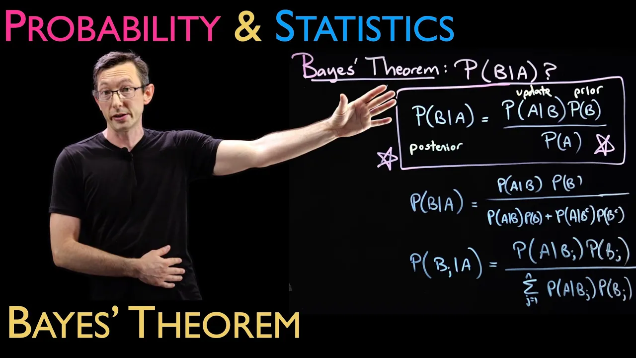
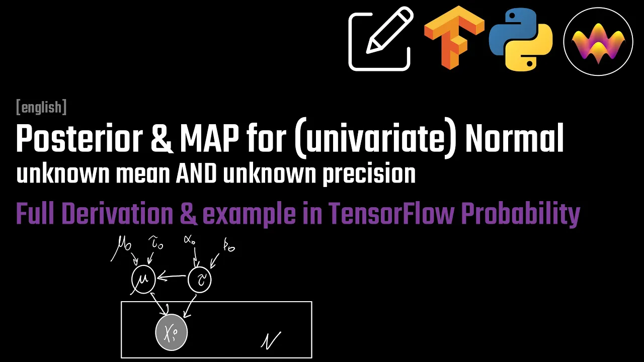
In Bayesian inference, when estimating an unknown mean μ with known variance σ², the posterior distribution is derived by multiplying the normal likelihood function with a normal prior distribution, then completing the square in the exponent to recognize the resulting distribution as normal with updated mean and precision. The posterior mean is a weighted average of the prior mean and the sample mean, where weights are proportional to their respective precisions (τ₀ and n), and the posterior precision equals the sum of the prior precision and the data precision (τ_post = τ₀ + n).
Bayesian Inference: Deriving the Posterior Mean & Precision
Added:Bayes' Theorem and its core components: understanding the mathematical relationship between the prior, likelihood, and posterior distributions.
The Normal (Gaussian) distribution, including its probability density function (PDF) and standard parameterization.
The concept of precision as the reciprocal of variance (1/sigma^2) and why it is mathematically convenient in Bayesian formulations.
The definition and utility of conjugate priors, specifically how they yield a posterior within the same probability distribution family as the prior.
Basic algebraic manipulation of exponents, specifically the technique of completing the square to identify the parameters of a normal distribution.
Joint estimation of both an unknown mean and an unknown variance/precision using a Normal-Gamma or Normal-Inverse-Gamma conjugate prior.
Multivariate Bayesian inference, extending the univariate normal model to handle vectors of means and covariance/precision matrices.
Bayesian Linear Regression, applying these derived posterior formulas to estimate regression coefficients with Gaussian priors.
Markov Chain Monte Carlo (MCMC) methods, learning how to handle non-conjugate priors where analytical posterior derivation is mathematically intractable.
Sequential Bayesian updating, demonstrating how the derived posterior acts as the new prior when a fresh stream of data arrives.
852 views4likes36:14Original Release: 2019-02-12
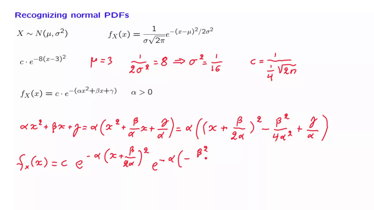
okay yeah so we're trying to stream the posterior derivation for the case where nu is unknown and Sigma is known so we have done it in the beta binomial case remember week likelihood we express the prior and then tried to the medical series should see if we can recognize in some way and so nor as you get there there's some algebra techniques that it's good you know so I'm going to do it give me some rules and let you do some practice so first of all let's work with the likelihood function so the likelihood function we know y1 to yn they're iid munch a new they're iid normal and so now the likely function remember likelihood is always in terms of function in terms of the unknown parameters and because no new is unknown it's a we express it just out you so where's mu so we know that there I I D so it's going to be the product of each of the individual density okay so let me write the PDF for you so in the biggest parentheses it's the density PDF of each observation why I the contribution and then because they're iid they're independent so the joint will be the product of all of them so I mentioned this to you earlier that while we usually understand normal in very me instead of aviation alarians it will be easier for us to think about something we call transition so let me just give you the definition together there's one over Sigma squared so it's the reciprocal of the variance so right now we're gonna work with this because it's easier for the derivation and then we can see the result in a clearer way right so that means we're going to replace the stigma in the likelihood function with 1 over 1 over C so let me so this means Sigma 1 all right so I'm gonna do that step for you and that has YouTube try next step so now is 1 over P a 1 over Sigma right so 1 over Sigma will be e to the power of half so Kony's yourself this is right so this is 1 over Sigma which will be the square root of all right so that's good and it's also pretty straightforward to do this one because you have 1 over 2 times 1 over Sigma square so that becomes B over 2 ok good so everything else stays the same and we simply replace their standard deviation with the precision and the one last step I will do for you please on the likelihood function is bring in flight they spend the terms decide the product I'm over here so this does not change with the index right so this the whole thing will just raise to collagen because your product and copies of them what do you have is and beat to the call Pat rage spell the end for me me to the pulp and over to you and what's important now is in the exponent so we know that if you product multiple exponential function together it's going to be a large exponential with all of the terms sum up together in it great so this is your raffle make sure that you weird so we can actually come to the term that it's gonna be the song and because she doesn't change by the index the only style that we're going over is a little review make sense okay so convince yourself that this is true and before I go to the prior distribution parts something good to keep in mind we're gonna come back to this again of course something good to keep you - like I said we like to use to recognize what is constant and then because once we know those who can throw them into the proportional sign so we don't have to worry about them needs a derivation too much okay so my question for you now is there are three terms one two three which are constant in terms of mu the first one constant right second one constant right third one because new is here so constant constant not constant okay so soonish what we are trying to derive the posterior you will see that those ghosts you go away we don't need them anymore so good you keep in mind I mean of course you stay afterwards with this part looks a little complicated but we're going to look at the job alright so this is the part let me also introduce you cheer the price so the prior distribution we know that use the precision instead of the standard deviation so we know that the prior from you is normal nu 0 and Sigma 0 so that's the setup that we had and again we put this in the conditional sign because it helps us to recognize that this is none and this is being commissioned alright so the prior distribution now is also a function so you notice we keep writing the function in terms of the only unknown parameter is the later we're going to use them to to drive the posterior so I'm going to write the density for you so now is Sigma 0 they need exponent this is just the regular NOLA density maybe you need to make sure that you get the correct mean under standard deviation so previously knew itself is the mean and Sigma itself is to standard deviation lately now it's a prior distribution for the unknown moon and we put a normal prior four edge with mean mu 0 and Sigma 0 so that's why the density PDF of knew in itself is in terms of Sigma 0 nu 0 and it's unknown so this definitely needs practice I mean it's easier it looks easy when people show you this for them when you're trying to derive it later might be pretty demanding so I'm trying to highlight the key steps so again would you find the precision I'm going to use a 0 which is 1 over Sigma 0 square so I'm going to use that for the later derivation I have one standard deviation with the position so before you move on the practice three terms which are constants first first you again write constant constant the third one is not conscious you better go away but then of course as you can see already that the third term not only here in the prior distribution we're also doing the likelihood it's kind of involved when you this resurrection previous was the foundation of of square term so there are some practice and good techniques over there that's what's going over and we're going to turn it try to do it now all right so posterior all right here remember I usually write the conditional probability distribution the data and so we know you should be proportional to the product of the prior and the likelihood so I'm going to write some terms for you and I give you some time to try to derive it and from the prior remember only the third term is not a constant so only that term matters right and I'll also write it for you that I should say I think it's this whole defeat and then sum of the Y I minus mu squared great I think that's what that posterior and the light dinners part that is not constant okay so this is collecting what we have previously so before I break to let you try it and maybe I should just do one more thing for you because remember when I show you what the Listeria is there's no more why I was expressed in terms of Y bar so that's actually a pretty standard practice when you're doing this kind of derivation for the normal normal conjugate prior practice so it's good to me let me show you good to recognize that okay so pretty much I'm trying to show you how to simplify this picture so later it's easier to see the results so I'm only going to focus what's either exponent for now so what I will be doing is I won't look at this part the reason why I'm doing it here as you can see soon because even though those two exponential terms inside as you in it but you also say in the first term you know it's mu zero right when you expand the squared term you have a squared nu 0 which is a constant so right now I'm trying to or we talked sure if you're trying to get rid of any unknown is not necessary constant in here that in the end we're only going to be left with terms about you as those going to help us to determine what's the posterior distribution so let's try to simplify this a little bit more so we only need to worry about the Nutri so we all do this I mean this is um and there exercise so I will just I will stop talking and do my art here you can try yours yes I expect some of the squared term in an exponent I mean yeah only the part like without the negative field or cheer for now and we can get the sum of Y squared minus 2 times n times y bar times of U plus n times nu squared ok so the first term it's about the data it's nothing about the new right so later as you can see that can go into the constant so that's why right now on the right when I in the in the green color I further simplify that to be proportional to the exponent of negative PI over 2 and only keeping mu square minus 2 and y bar mean we're going to use this later when we derive it so the green all right in the bottom is trying to give me it's a short term it's a demonstration of how to further by it in terms of new square all right so I'm going to raise this part then I will give you a few minutes to complete this square so what I mean by complete the square is now I mean there is still some work you can do with the first exponent from the prior right cuz it's negative V 0 over 2 times mu minus mu 0 squared so if you expend a squared term you will give you square right negative 2 mu mu 0 plus mu 0 squared mu 0 square should go away go into the proportional time because it's a constant so trying to do that and I will stop talking for a little bit try to do that and you will start to recognize that for both exponent terms you have something about you square you have something about you you combine those terms you might be able to recognize what the distribution is and so I'm going to pause for a few minutes take your time this is I mean specially the first time seeing this will be a little bit stretching of your tubes and practice so take your choice and we're not in a hurry to choose lunch the goal again it's trying to only have the terms about mu 0 where mu squared and you from there you might be I know some of your working I should just use one more thing is once you arrive at some place what I mean by comfort is where it suits number the distribution is so generically you know that you have ax squared plus BX plus some constant you're able to company the squared great so what I would do is that I'm having on this row so this is what the eight X plus a constant right and I get 4x plus I think it's B over 2a right squared right and then the still plus the constant even I mean the see they have to - hey this is a start practice by completing and squared so I'm mentioning this because as you know identity of the normal is 1 in the explanation if Y follows normal Mu Sigma then this do fly I mention we're lectures because once you have done the further we say trying to simplify further simplification of this two terms now we know is 2 exponent turns multiplied together right so they can be combined into one with the sum of the inner parts so once you do that you will have some terms of nu squared I have some term of mu and if you complete the square you might be able to recognize what's the new mean should be because that would be a posterior meet because I already said the posterior is a normal distribution right so now we have most of the terms there the goal is to make sure that you can recognize and the after simplification your correct place what will be the MU in the posterior and of course the Sigma square in the posterior I already showed the results but I bet you don't remember anyway LSU wrote it down this is complicated but if you keep doing this we're going to pause for a few more minutes I want to mention why what I mean by complete the square and the generic form is this and the goal is to help us to recognize this so of course in the normal in a normal tournament I mean it's going to be a negative sign over here I'm saying you will be able to recognize this B or issue a is now whatever is multiplied beforehand will be related to two standard deviations so take your time and I'm gonna pause for it for a little one I just want to share with the hint right you get to this point but this is for the simplification and combine the terms of new Sigma Nu square and new so in front of nu square it's negative 1 over 2 times p0 plus n times P and if I know from you it is 1 over 2 nu 0 T 0 plus 2 times M Y bar times B and then the last step in the next episode is company that's where I'm going to do to show you the results here [Music] [Music] [Music] so I will share notes afterwards of course so no are too much fun but I do want you to do it in skills in the normal case so this is after you complete the square this is what you get and just like what I wrote earlier if you look at the Rolo density you can start to recognize what is the mean coasteering mean what's the posterior standard deviation right so close dear to me is whatever is in the square term that is being subtract from unknown you right so close dear I mean is UN and this part remember if we express the normal PDF in terms of precision this is exactly what is being multiplied before the squared term right so this should be what yeah or or if you guess so for the position because your position will be will be this and then the posterior standard deviation will be one over this and then square root right ultimately we have the posterior be normal so the mean is what we have over here is we win so it's V 0 mu 0 plus NY bar we divide it by G 0 plus mg right and then the standard deviation is 1 over 0 plus and C and that's why I showed you earlier on the slide so details obviously you might want to go back to yourself but ultimately you I mean the key to you I'll be here I think it's making sure that you get the right terms recognize what it's constant yeah but you throw it away into the proportional sign and then of course in the end complete the square and the reason why we complete the square just because our goal is trying to recognize what is the density for this and as you can see we again you use the all of this no sorry right so for this case we won't go into the detail keeping those constant and trying to show that it is indeed normally there's too much work but just please make sure that you are able to follow what we showed in class today using the proportional sign and be convinced that in the end you do come to a normal Dennis Dean this way so I wish your notes afterwards so don't worry so I'm going to clean this now and bring back to the slide that we have here so this is exactly the evolution 14 that was a revelation exercise that we did so we have two more minutes left the only thing I want to talk about is just looking at looking at the posterior I mean for a second so in the beta binomial case I show you that the posterior view is a weighted average of the prior me and the sample mean right so I want you to do the same practice here so obviously prior me is this right sample mean you can think of it as is y bar but you can also think about it as I mean simple sum in some sense because that's all the contribution together so you can see that in the numerator is 0 times the prior me plus fee times to example me or the data mean right no I think it's sorry I think it's easier to just recognize the sample mean sorry about that to just focus in one sample me so this is the weight part of the weight right and I should say they started the part of the weight and times B and as you can see in the denominator is the sum of this two so why are the weights the weights from you zero is a 0 over T 0 plus n 0 okay and the weights for y bar is empty over to 0 plus empty so again the posterior mean is a weighted average of the prior me and the sample mean and that of course how largest be 0 largest fee and how large is the sample size going to play an important role in terms of how much of contribution to the posterior mean is from the prior me and from the sample and n which is the sample size obviously as n grows bigger a contribution of Y bar s speaker and this also reinforces our idea that if you have a larger sample or have larger amount of data the data are going to start to dominate the posterior so this again as you can see I mean this is the same sort of like similar similar approach sorry you think about the whole structure that at the beginning we talked about how the prior and the data contributes to posterior and then in specific model like beta binomial and here we call this normal normal model because the normal density and then you put a normal conjugate prior normal and in this case in those in the way that we okay
Up Next

11:04
Normal Prior Normal Likelihood Posterior Derivation
@deetoher
57.2K views•2013-03-08

4:43
Elliptic Curve Cryptography Explained: ECC, ECDSA, ECDH
@PracticalNetworking
28.5K views•2024-10-21

10:44
Fourier Series Introduction: The Big Idea Explained
@DrTrefor
387K views•2021-05-03

6:00
The Mathematical Impossibility of Accurate World Maps
@Vox
23.3M views•2016-12-02
Related Study Plans & Knowledge Roadmaps
Structured learning paths in Mathematics
mathematics
Tensor Calculus: Vectors to Riemann Curvature
01Mathematical Foundations: Linear Algebra & Calculus
02Covectors, Dual Spaces, and Tensor Basics
03The Metric Tensor and Index Gymnastics
+ 2 more learning modules
40h5 modules
Explore Roadmap
mathematics
Gödel's Incompleteness: Logic, Proofs & Limits
01Introduction to Formal Systems & Hilbert's Dream
02Set Theory, Cardinality, and Cantor's Diagonal Argument
03Arithmetization and Gödel Numbering
+ 2 more learning modules
14h5 modules
Explore Roadmap
mathematics
Galois Theory: Fields, Groups & Solvability
01Foundations of Abstract Algebra: Groups & Fields
02Polynomials & Field Extensions
03Splitting Fields & Symmetries
+ 2 more learning modules
24h5 modules
Explore Roadmap
mathematics
Non-Euclidean Geometry: Models & Geodesics
01Euclid's Fifth Postulate and the Birth of New Geometries
02Hyperbolic Space and the Poincaré Disk Model
03Geodesics: Defining Straight Lines in Curved Spaces
+ 2 more learning modules
15h5 modules
Explore Roadmap