
















![[20230517] 3.5 다변량 정규분포 및 행렬대수(전치, 행렬식, 고유값과 고유벡터) 복습 / 3.6 t분포와 F분포의 정의, 스튜던트 정리](https://i.ytimg.com/vi/3SbZm1_cOf0/maxresdefault.jpg)
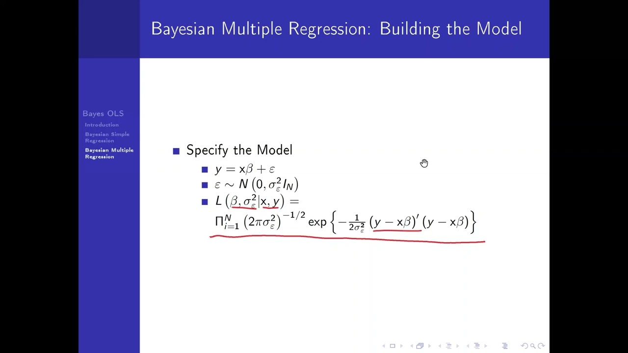







When a normal distribution serves as the prior for a normal likelihood function, the resulting posterior distribution is also normal, with its precision equal to the sum of the prior precision and the likelihood precision, and its mean being a weighted average of the prior mean and the sample mean, where weights are proportional to their respective precisions.
Normal Prior Normal Likelihood Posterior Derivation
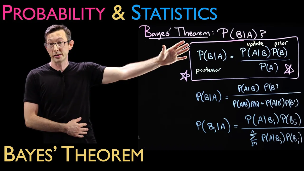
Added:Understanding of Bayes' Theorem, specifically the relationship where the Posterior is proportional to the Likelihood multiplied by the Prior.
Familiarity with the Probability Density Function (PDF) of the Normal (Gaussian) distribution and its parameters (mean and variance).
Algebraic proficiency in 'completing the square' within the exponent of exponential functions.
The concept of 'precision' in statistics, defined as the reciprocal of the variance.
Exploring the Multivariate Normal conjugate update, extending this univariate derivation to multi-dimensional data using matrix algebra.
Applying the Normal-Normal model to Bayesian Linear Regression, where priors are placed on the regression coefficients.
Studying Conjugate Priors and the Exponential Family to understand which other distribution pairs share this convenient property.
Implementing Sequential Bayesian Updating, demonstrating how a posterior distribution becomes the prior when new data is observed.
57.2K views397likes11:04Original Release: 2013-03-08
so now we're going to look at the likelihood based on N samples from a normal distribution so n mu Sigma squ and we've already shown that that's distributed normally with a mean of the sample mean variance of Sigma n now if we have a prior recalling that the product of gaussian or normal distributions is also a Galan normal distribution it's not a bad idea to have our prior also to be a normal distribution because then we're going to have a normal distribution times a normal distribution the result will be a normal distribution so we're going to say it's some mean and some variance the prior times the likelihood will be normal with some mean I'm denoting mu n and some variance I'm denoting Sigma n^ 2 as We Know s s and n and sigma squ we can ignore the constant term and this constant term is of the form of 1 over the square root of 2 pi Sigma SAR to the power of n * 1 over the < TK of 2 pi S 2 and it's so it's of this type of form proportional to that they're all constants we can ignore that we have G of mu y1 Over N there 2 YN is proportional to the prior times the likelihood given the data so we say it's proportional to the exponential part because we're ignoring the constant bit of our mean of our prior which Sol the form with respect to M and mu so we're going to have -1 / 2 s^2 mu - M to b ^ 2 time the exponential of 1us it's not no longer it's 1/ 2 Sigma s / n so it becomes on top time mu - Y Bar to b^ squ well you can remove this bit here and just add them together and expand out the brackets which is equal to the exponential of -1 / 2 s^ 2 mu^ 2 + m^ 2 - 2 mu M - n / 2 Sigma 2 mu^ 2 + Y bar^ 2 - 2 mu Y Bar so we then progress on and we group the terms containing the similar powers of mu together so it's equal to exponential of Min -1 /2 and we'll keep that outside for convenience mu^ 2 time well 1 / S 2 the minus has been dealt with so plus n over Sigma squ now we'll look at the terms containing mu to the^ of 1 and they both have additional minuses so - 2 mu then we have M over s² plus cuz we have sufficient minuses to deal with everything N Y Bar over Sigma 2 and then we actually have plus stuff that doesn't depend on mu so we don't actually have to be too concerned about it but for completeness we'll have it's m^2 over S 2 + Y bar^ 2 over Sigma 2 now we expect to see something of the form exponential - 1/ 2 Sigma 2 N into mu^ 2 + mu n^ 2 which we're going to be not too bothered about mu mu n so we'll concentrate on matching the powers of mu s of mu not of mu n but only of mu so we have minus 1 / 2 Sigma 2 n * mu is equal to -1 / 2 mu and sorry squared mu^ 2 1 / s^ 2 + n / Sigma 2 and you'll see here this implies that 1/ Sigma s is equal to 1 / s^ 2 + n/ Sigma 2 so this is the Precision of your posterior is equal to the Precision of your prior plus the Precision of your likelihood this should be in here so we also note that 1/ Sigma 2 N can also be written in the form of Sigma 2 + s^ 2 N / by Sigma s s² which implies that Sigma SAR n is equal to Sigma 2 s^ 2/ Sigma 2 + S Square n so this will become clear later on as to why we bothered to do this so the next part is we've expected to see the next part we've expected to see is in terms of our y ends is we have minus 2 it's minus by minus becomes a plus mu mu n over 2 Sigma n^ 2 is equal to Mu mu n over Sigma 2 N and we want to compare it to our term with mu^ 2 with with just mu in it and that's going to be equal to well the twoos above and below the line cancel the minuses and minuses become a plus so it's equal to mu * m / S 2 + n y bar/ Sigma 2qu canceling your M's you get mu n / the variance of our posterior is equal to M Sigma squ + n y s 2 / Sigma 2 s s now so mu n is so that's the mean of our posterior is equal to Sigma 2 n * mu or M Sigma 2 + n y s 2 / Sigma 2 S 2 which if we recall from earlier why did I bother to put it into this form so it's equal to Sigma 2 S2 over Sigma 2 + S 2 n * m Sigma 2 + N Y Bar S 2 / Sigma 2 S 2 and we get things that cancel quite nicely so you get that the mean of the posterior is m Sigma 2 + n y s 2 over Sigma 2 + s^2 n now for convenience we actually tend to write this of the form Sigma 2 over Sigma 2 + S 2 n * m + S 2/ Sigma 2 + S 2 n n y bar remember that's just your sum of your values
Up Next
25:02
MCMC Explained: Bayesian Sampling and Convergence (Oxford Talk)
@teachingandlearningmathematics
6.6K views•2024-04-03

4:43
Elliptic Curve Cryptography Explained: ECC, ECDSA, ECDH
@PracticalNetworking
28.5K views•2024-10-21

10:44
Fourier Series Introduction: The Big Idea Explained
@DrTrefor
387K views•2021-05-03

6:00
The Mathematical Impossibility of Accurate World Maps
@Vox
23.3M views•2016-12-02
Related Study Plans & Knowledge Roadmaps
Structured learning paths in Mathematics
mathematics
Tensor Calculus: Vectors to Riemann Curvature
01Mathematical Foundations: Linear Algebra & Calculus
02Covectors, Dual Spaces, and Tensor Basics
03The Metric Tensor and Index Gymnastics
+ 2 more learning modules
40h5 modules
Explore Roadmap
mathematics
Gödel's Incompleteness: Logic, Proofs & Limits
01Introduction to Formal Systems & Hilbert's Dream
02Set Theory, Cardinality, and Cantor's Diagonal Argument
03Arithmetization and Gödel Numbering
+ 2 more learning modules
14h5 modules
Explore Roadmap
mathematics
Galois Theory: Fields, Groups & Solvability
01Foundations of Abstract Algebra: Groups & Fields
02Polynomials & Field Extensions
03Splitting Fields & Symmetries
+ 2 more learning modules
24h5 modules
Explore Roadmap
mathematics
Non-Euclidean Geometry: Models & Geodesics
01Euclid's Fifth Postulate and the Birth of New Geometries
02Hyperbolic Space and the Poincaré Disk Model
03Geodesics: Defining Straight Lines in Curved Spaces
+ 2 more learning modules
15h5 modules
Explore Roadmap