


![BUS 6010 2 - 3 ส.ค. 57 [3] 20140803080645](https://i.ytimg.com/vi/j-YKwi90FD0/sddefault.jpg)



![[객관식 공기업 경제학] 25차시_기8공_경제학_거시편_제4편_IS-LM모형과 경제안정화정책 (1)_516~537](https://i.ytimg.com/vi/5U40xhB0Ow0/maxresdefault.jpg)










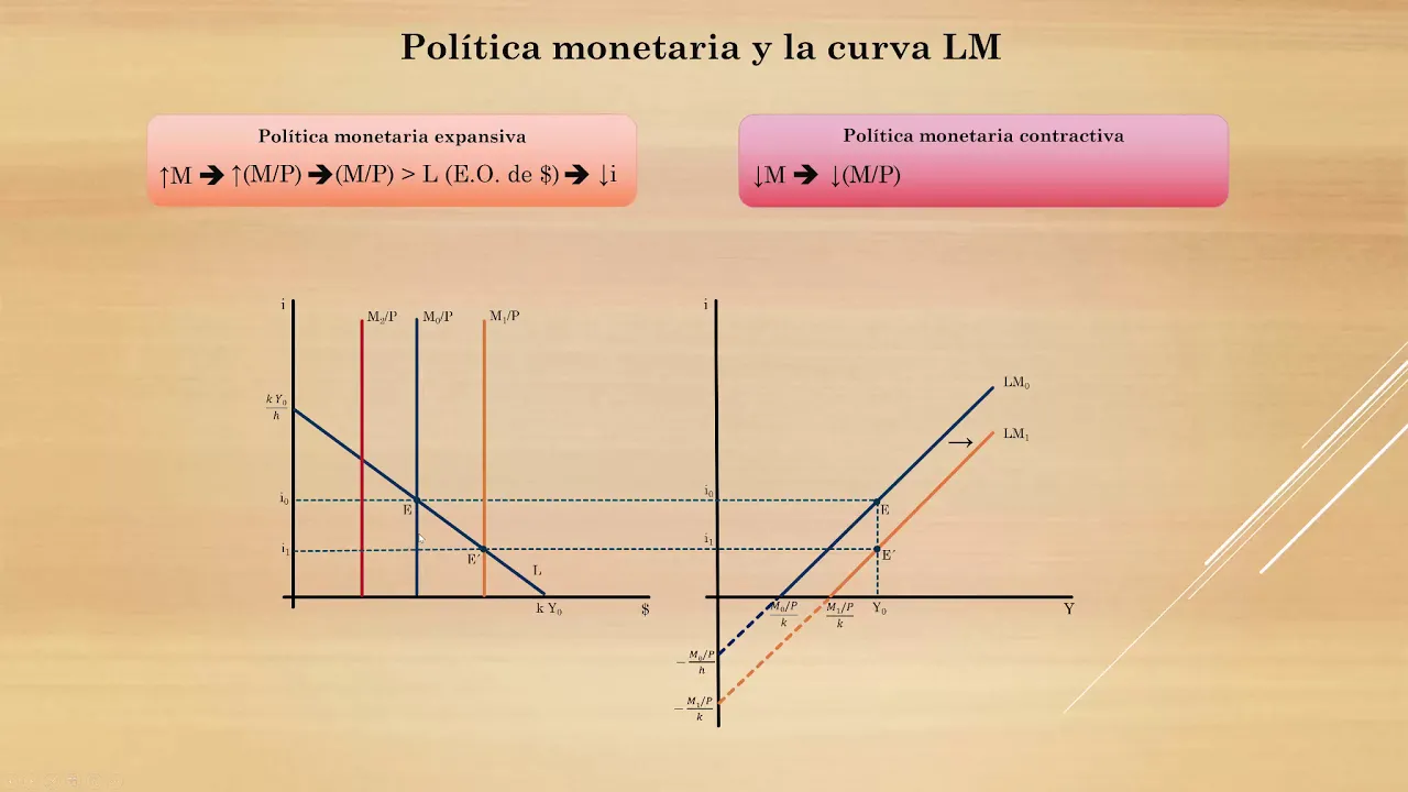
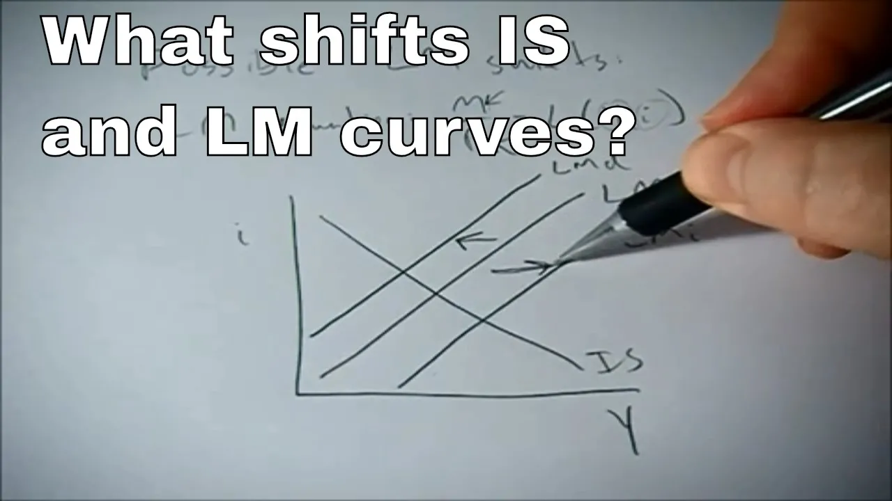


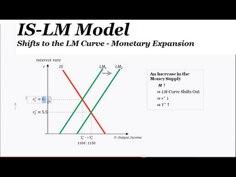

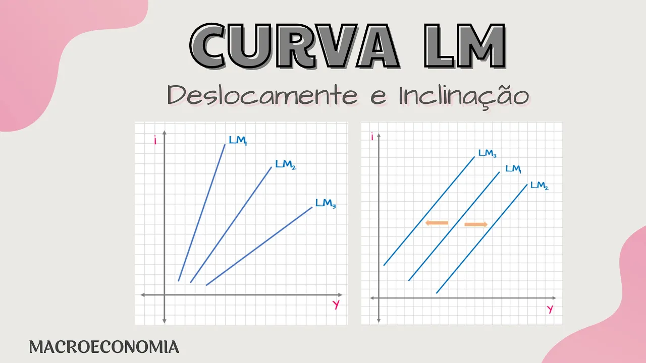





The LM curve represents money market equilibrium in the ISLM model, showing the combinations of interest rates and output levels where money demand equals money supply. Money demand consists of two components: transactions demand (ky, positively related to output) and speculative demand (-lr, negatively related to interest rates). The money supply is M̄/P (nominal money supply divided by price level). Setting money demand equal to money supply yields the LM curve equation: r = -(M̄/P)l + (k/l)y, which has a positive slope (k/l) and negative vertical intercept. Graphically, the LM curve is derived by plotting transactions demand (upward sloping from origin) and speculative demand (downward sloping), then finding equilibrium points where their sum equals money supply, resulting in an upward-sloping curve in the r-y plane.
ISLM Model Part 3: Deriving the LM Curve Mathematically & Graphically
Added:[Music] so now we come to the derivation of the lm curve now as i've already stated in the introduction the lm focuses on the money market equilibrium and by the virtue of all we can see that if the money market clears the bond market will definitely clear so the lm curve is showing the equilibrium situation in the wealth market as a whole so the lm primarily focuses on the money market equilibrium and by the virtue of already law it shows the bond market equilibrium in order to show the money market equilibrium first of all we need to understand what exactly the money demand is actually the money demand can be divided into two parts one part is known as the transactions demand for money and the second part is known as the speculative demand for money now what do these two components mean transactions demand is simply equal to k into y it is having a positive relation with output where y is the output and k is a positive constant so if y increases the transactions demand is also going to increase the speculative demand for money on the other hand is dependent on the rate of interest and it has got a negative relation when plotted with respect to r so this l is a positive constant and the slope of the speculative demand curve is minus l which implies that it is having a negative relation with r so these are the two components of money demand and the money supply in the economy is equal to m bar by p now the point is why are we considering the money supply to be equal to m bar by p actually this m bar is the nominal supply of money it is the supply of money which is fixed by the central monetary authority of the country and p is the general price level of the goods and services so the nominal money supply divided by the price level will give us the real supply of money in the economy and for the money market to be in the state of equilibrium the condition is money demand should be equal to money supply so from here we are getting ky minus lr is equal to m bar by p now simply making some modifications and adjustments in this equation we will get r equals to minus m bar by p into l plus k into y by l this is what the equation of the lm curve is it has got a positive slope which is equal to k by l and it has got a negative vertical intercept which is equal to minus m bar by p into l when plotted in the r y plane so this is what the mathematical form of the lm curve is so now we come to the graphical approach of deriving the lm curve now we need the two components of money demand for the graphical derivation the transactions demand which i have already described it is equal to ky and the speculative demand is equal to minus lr we will be using a four panel diagram where we will be linking these two components and we will be plotting the lm curve in the r y plane the four panel diagram that we are considering it will be such that in the first quadrant in the horizontal axis we are recording output and in the vertical axis we are considering r in the second quadrant here we will be recording the values of speculative demand and along this particular axis we will be recording the values of the transactions demand for money now the point is how exactly does the transactions demand curve look like the transactions demand is equal to k into y so it is a positively sloped function with respect to y because k is a positive constant and at the same time if output or y is equal to zero transactions demand will also be zero so it will simply be an upward sloping origin passing straight line in the y trdd plane that means if y increases transactions demand also increases so this is your transactions demand curve now come to the speculative demand curve the speculative demand curve as i have already shown is having a negative relation with r because l is a positive constant so if this increases the rate of interest increases the speculative demand is going to fall so from here we can see that the speculative demand curve will be negatively sloped if r increases the speculative demand is falling so this is what the speculative demand curve is in this quadrant or the third quadrant we will be drawing a line which will have equal vertical and horizontal intercepts that means this intercept will be equal to this intercept this line will basically ensure that the total money demand is equal to the addition of the speculative demand and the transactions demand because this vertical and horizontal intercepts that we are considering they will be equal to m bar by p so the point is if this intercept is also m bar by p and this intercept is also m bar by p if you consider any particular rate of interest suppose we are considering this r0 corresponding to r0 the value of the speculative demand for money will be at this level if the value of speculative demand for money is at this level the value of transactions demand for money will be at this particular level and if the value of transactions joined for money is at this level the value of output will be at this level now as i was telling why we are considering this line in such a way that it is having equal vertical and horizontal intercepts this is because you see when the rate of interest is r0 corresponding to r0 the speculative demand for money is this much if this much is the speculative demand for money that implies this value is also equal to the speculative demand because this is a rectangle after all so this particular value and this particular value both are equal if this is the speculative demand for money then we can say that this particular value this remaining portion that will be the transactions demand for money because at equilibrium the money demand is equal to money supply and the money supply is nothing but m bar by b so if this component is equal to the speculative demand for money the remaining component will be equal to the transactions demand for money such that their sum is equal to m bar by b which is the money supply in the economy so corresponding to this value of r we are getting the speculative demand and from the speculative demand we can easily find out the transactions demand and corresponding to the transactions demand we can find out the value of y uh say the value of y is equal to y0 now if the rate of interest rises say to r1 corresponding to the new rate of interest r1 we will see that the value of speculative demand is somewhere around here if the value of speculative demand is this then the value of transactions demand will be the remaining part because the total intercept is the money supply so if this is the speculative demand this remaining portion will be the transactions demand this portion and this portion both will be equal because this will be an isosceles triangle so if this is the transactions demand this is also the transaction statement and we can also see that corresponding to this value the value of the transactions demand is also equal to this and this length and this line both are equal so if this is the transactions demand you will get the new level of output as y1 so corresponding to the rate of interest r1 you will see that the output in the economy is y1 if you simply join this point and this point you will get the ln curve which is upward sloping in the ry plane so just by combining the money market equilibrium situation we can easily obtain the lm curve in the ry plane and the ln curve as we saw in the mathematical form is upward sloping and it has got a negative vertical intercept so this is what the graphical form of deriving the lm curve is [Music] you
Up Next

Open Economy IS-LM & Mundell-Fleming Model: CUET Economics
@ravitthukralhaqseeconomics
579 views•2024-03-03

Impact of Yuan in Indo-Russian Trade Amid Sanctions
@WION
261.9K views•2022-07-01

Behavioral Economics Explained: Rationality, Nudges, and Risk
@crashcourse
1.1M views•2016-03-12

The Age of Easy Money: Fed & Inflation | Full Documentary
@frontline
21.2M views•2023-03-15
Related Study Plans & Knowledge Roadmaps
Structured learning paths in Economics