



























The mean (expected value) of a continuous probability distribution is calculated by integrating x multiplied by the probability density function (PDF) over all possible values, while the variance is derived using the relationship Var(X) = E[X²] - (E[X])², where E[X²] is found by integrating x² times the PDF. For example, with a PDF f(x) = (1/60)x³ defined between 2 and 4, the mean is approximately 3.3 and the variance is approximately 0.266.
Deriving Mean and Variance of Continuous Probability Distribution
Added:Fundamental concepts of single-variable integral calculus, including integration by parts and evaluating improper integrals.
The definition and mathematical properties of a Probability Density Function (PDF) for continuous random variables.
The conceptual understanding of mean (expected value) and variance in the context of discrete probability distributions.
Basic algebraic manipulation and the mathematical properties of expectations, such as the linearity of expectation.
Deriving the mean and variance for specific standard continuous distributions, such as the Uniform, Exponential, and Normal distributions.
Introduction to Moment Generating Functions (MGFs) as an elegant, alternative method for finding the moments of continuous distributions.
Calculating higher-order moments of continuous distributions, specifically skewness (third moment) and kurtosis (fourth moment).
Exploring joint continuous probability distributions, which includes finding covariance, correlation, and conditional expectation.
Applying mean and variance to key statistical theorems, such as Chebyshev's Inequality and the Central Limit Theorem.
338.4K views4Klikes7:22Original Release: 2012-12-28
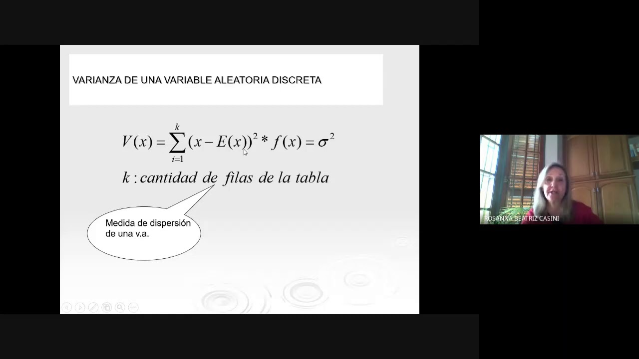
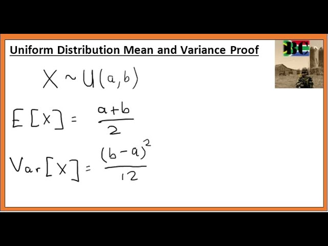
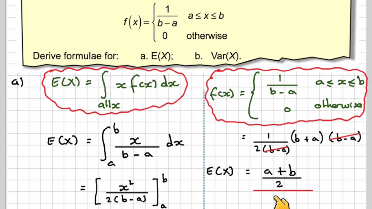
let's look at deriving the mean and variance for continuous probability distributions this does require some calculus and I'm going to assume that you are familiar with basic integration suppose for a random variable X the PDF f ofx is equal to 1 60 * X cubed when X is between 2 and 4 and Zer otherwise let's take a look at what that looks like here's the PDF plotted out this curve is 1 60 * X cubed between 2 and 4 and then it drops to zero outside of that range of values suppose the point of interest for us is finding the mean and variance of this probability distribution here I've written out the PDF and we're looking for the mean of the probability distribution I've written out the expectation of X here which is another name for Mu the mean of the distribution for a continuous random variable the expectation of X is equal to the integral from minus infinity to Infinity of x * F ofx DX here we're going to integrate x * 1 60 x Cub DX but we're not going to integrate this between minus infinity and infinity because this is only the PDF between 2 and 4 outside of 2 and 4 it's zero so we integrate this between 2 and 4 because the integral from minus infinity to 2 is zero and from 4 to Infinity is also zero this is going to be equal to 1/ 60 time the integral from 2 to 4 of x to 4th power DX this is equal to 1/ 60 * when we integrate x 4th we get X 5th over 5 and we need to evaluate that between 2 and 4 so if we come up here this is going to be equal to 1/ 60 * 4 5th power over 5 - 2 to the 5th power over 5 and this works out to 992 over 300 and in reduced form if we were to reduce that we'd see that this is 248 over 75 which is approximately 3.3 and that is the mean of the distribution if we go back to our plot of the PDF we' have three right in the middle here and we would see that values near Four are more likely than values near near two and that draws the mean over here to about 3.3 that's our mu our mean of this probability distribution now let's derive the variance of this probability distribution the variance Sigma s is equal to the expectation of xus mu ^ 2 the average squared distance from the mean and to find this expectation we simply take this function and multiply it by the PDF and integrate over the possible values of X we could go ahead and find our variance in this manner we could Square this out and carry out the integration and find our variance like this however it is a little bit easier if we use a very handy relationship here in that the expectation of xus mu^ SAR is equal to the expectation of the square of x minus the expectation of X all squared this is a very handy relationship that we use in a lot of spots it might not be obvious that this is true just looking at it but it can be shown simply by squaring this out and using some properties of expectation now one of the reasons why this is easier is that we've already found this value so when we're finding the mean and then the variance we've found this one already so the question boils down to finding the expected value of the square of X so let's go ahead and find this the expectation of the square of X is going to be equal to the integral from minus infinity to Infinity of x^2 * FX DX and this is going to be equal to the integral of x^2 * 1 60 x cubed DX but again using a similar argument to the last time it's only this in between two and four and outside of that range of values it's zero so we integrate this function between 2 and 4 and this is equal to 1 60 * the integral from 2: 4 of x to the 5th power DX and if we carry out this integration we're going to get 1/ 60 * the integral of x 5th power which is going to be x to the 6/ 6 and we're going to be evaluating that between 2 and 4 and so this is equal to 1 60 * 4 6/ 6 - 2 6/ 6 and this works out to 4,032 2 over 360 and if we reduce that we'd see that's equal to 56 over 5 and recall again what we just found was the expectation of the square of X now let's go ahead and find the variance of this distribution the variance of the distribution which is equal to the expectation of x - mu^ 2 is also equal to the expectation of x^2 minus the expectation of X all squar and we found these values we just found that the expectation of x^2 is 56 over 5 and previously we found that the expectation of X is 248 over 75 that's what we found first and we're squaring that and this if we work that out is equal to 1496 over 5625 which is approximately to three decimal places anyway 0.266 and that's how we go about deriving the mean and variance of any continuous probability distribution
Up Next
12:04
Random Variables Explained: Discrete vs Continuous | Probability
@khanacademy
1.1M views•2009-02-16

4:43
Elliptic Curve Cryptography Explained: ECC, ECDSA, ECDH
@PracticalNetworking
28.5K views•2024-10-21

10:44
Fourier Series Introduction: The Big Idea Explained
@DrTrefor
387K views•2021-05-03

6:00
The Mathematical Impossibility of Accurate World Maps
@Vox
23.3M views•2016-12-02
Related Study Plans & Knowledge Roadmaps
Structured learning paths in Mathematics
mathematics
Tensor Calculus: Vectors to Riemann Curvature
01Mathematical Foundations: Linear Algebra & Calculus
02Covectors, Dual Spaces, and Tensor Basics
03The Metric Tensor and Index Gymnastics
+ 2 more learning modules
40h5 modules
Explore Roadmap
mathematics
Gödel's Incompleteness: Logic, Proofs & Limits
01Introduction to Formal Systems & Hilbert's Dream
02Set Theory, Cardinality, and Cantor's Diagonal Argument
03Arithmetization and Gödel Numbering
+ 2 more learning modules
14h5 modules
Explore Roadmap
mathematics
Galois Theory: Fields, Groups & Solvability
01Foundations of Abstract Algebra: Groups & Fields
02Polynomials & Field Extensions
03Splitting Fields & Symmetries
+ 2 more learning modules
24h5 modules
Explore Roadmap
mathematics
Non-Euclidean Geometry: Models & Geodesics
01Euclid's Fifth Postulate and the Birth of New Geometries
02Hyperbolic Space and the Poincaré Disk Model
03Geodesics: Defining Straight Lines in Curved Spaces
+ 2 more learning modules
15h5 modules
Explore Roadmap