







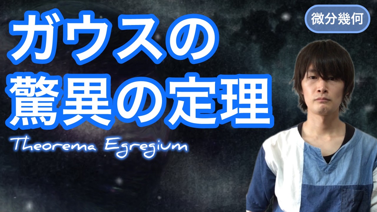



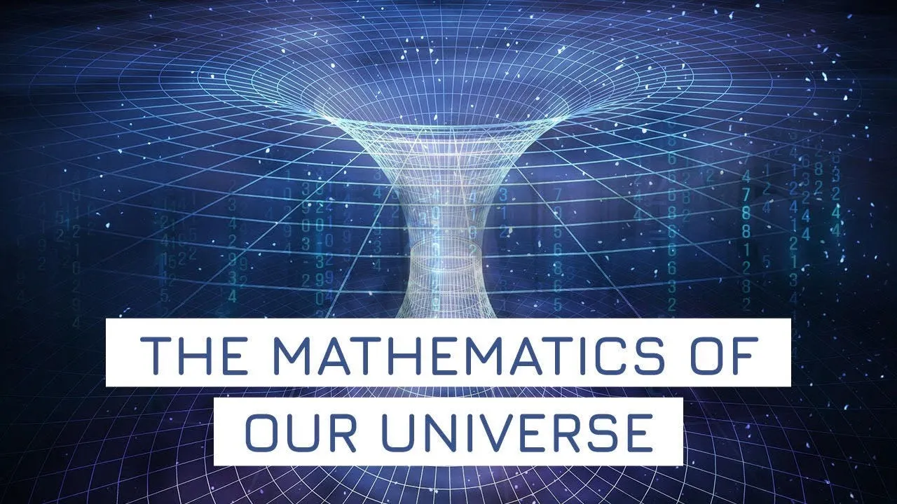
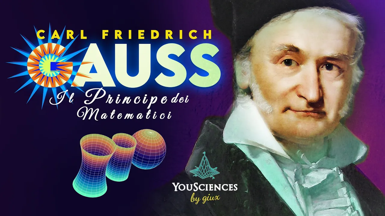


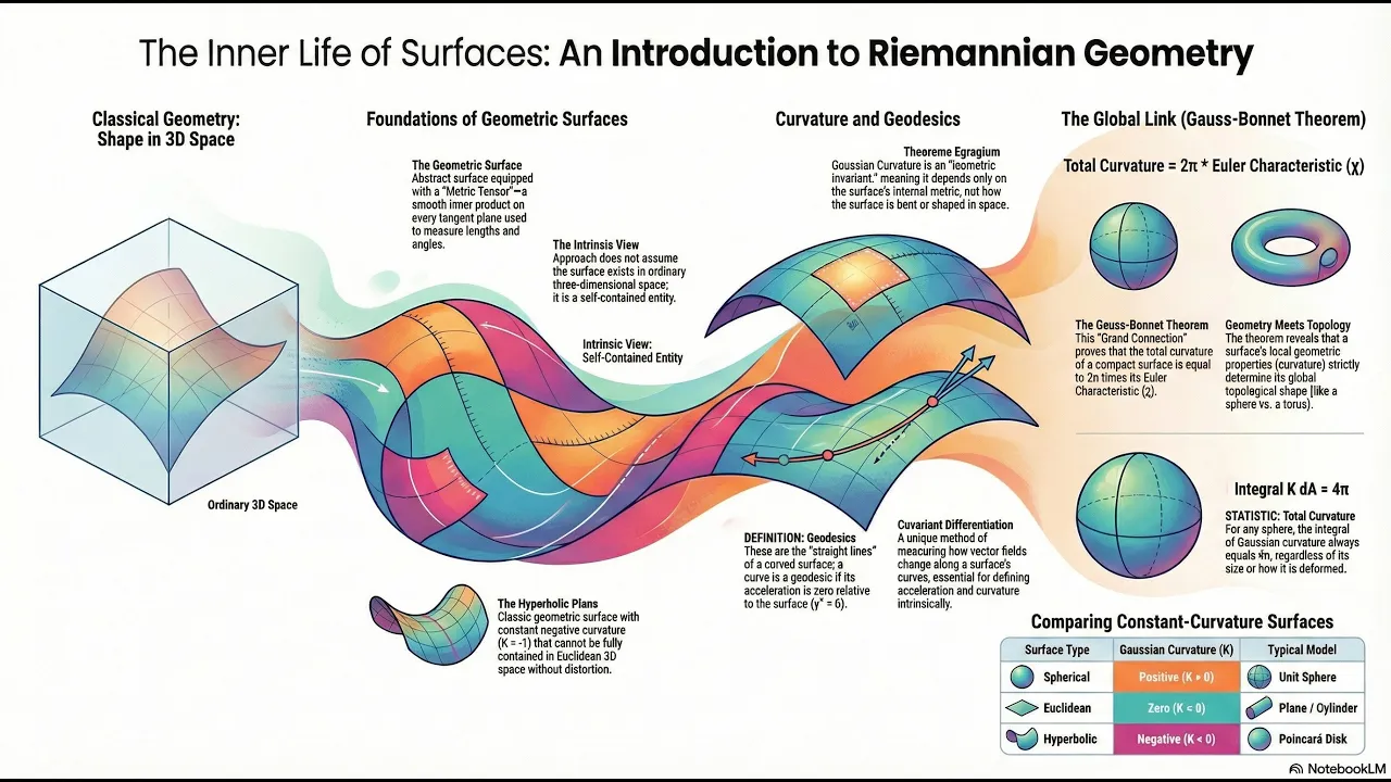





The Theorema Egregium (Remarkable Theorem) by Carl Friedrich Gauss demonstrates that the curvature of a surface is an intrinsic property that can be determined solely from measurements taken entirely within the surface, without reference to the surrounding three-dimensional space; this theorem establishes that the Gaussian curvature remains invariant under isometric deformations (such as bending a sheet of paper without stretching it), fundamentally changing our understanding of geometry and leading to the development of differential geometry.
Theorema Egregium I: Curves & Curvature in Differential Geometry
Added:Multivariable Calculus: A strong grasp of vector-valued functions, parametrization of curves, limits, and partial differentiation.
Linear Algebra: Familiarity with vector operations such as dot products, cross products, norms, and linear independence.
Introductory Real Analysis: An understanding of the formal definition of arc length, limits of integration, and differentiability.
Surfaces and Fundamental Forms: Transitioning from 1D curves to 2D surfaces, and learning about the First and Second Fundamental Forms.
Gaussian and Mean Curvature: Exploring how curvature is defined for surfaces, distinguishing between intrinsic and extrinsic properties.
Gauss's Theorema Egregium: Rigorously proving that Gaussian curvature is an intrinsic property that is invariant under local isometry.
Geodesics and the Gauss-Bonnet Theorem: Understanding the shortest paths on curved surfaces and how local geometry dictates global topology.
Applications in Physics and Graphics: Applying these geometric principles to General Relativity (spacetime curvature) or 3D computer graphics and mesh processing.
144.2K views2.3Klikes28:36Original Release: 2023-09-05
foreign [Music] the most remarkable theorem part 1 curved space [Music] Germany around 1787.
[Music] a young Carl Friedrich Gauss sits in his grade school classroom and Ponders the solution to an arithmetic problem on the board add all the counting numbers from 1 to 100 together that should surely keep the students busy While others around him would scratch away calculations on their slate boards Gauss began to visualize his solution a pattern amongst the problem within minutes you had a solution the answer came to him he imagines adding the same list of numbers to itself backwards this in turn produces 100 copies of the number 101.
so 10 100.
but since this is doubled the value that we actually needed dividing this number by two gave him the solution in minutes ten-year-old Gauss Returns the answer to his teacher of 50 50.
this would be the beginning of gauss's demonstration of his genius amongst the many things that he did throughout his life he proved the constructability of the regular 17 gone something that had eluded the ancient mathematicians for hundreds of years [Music] and among his other achievements Gauss is responsible for the fundamental theorem of algebra which connects the degree of a polynomial equation to the number of solutions that it can have and although this result would be enough to solidify gauss's name in the mathematics history this would pale in comparison to what he would develop while working as a surveyor to measure the Earth he invented the heliotrope in order to make accurate measurements of distances and during this time as a surveyor he would develop concepts of the least squares approach to finding the line of best fit later he would develop areas of statistical analysis by exploring normal or gaussian bell curve distributions perhaps though it was the difficulties of measuring surveyed curved surfaces that led him to the discovery of what he would call in Latin the theorima agreedium or the remarkable theorem a theorem that would blossom into the study of differential geometry now in order to make a map one must measure angles distances and areas accurately so what is the problem with making a good map well for one maps are typically flat and the world is not it's curved and so are the paths traveled around it so just how do you flatten a sphere many attempts at making Maps flat brought to light a simple problem when you flatten a map something gets distorted here is the well-known Mercator map and what is good about it is that it preserves angles [Music] but areas become distorted when you move closer to the poles now other maps have been put forward for instance one called the gall Peters map which preserves areas but angles get distorted instead and so that changes the point of view from someone navigating with such a map in fact here's a picture of the gulp heaters map so although it accurately depicts the size of land masses going in certain directions would be difficult because angles are not preserved and so we are now led to the conclusion that we must get a better understanding about how curved surfaces work by examining curved paths known as parametric curves [Music] coordinates of a point along a curve can be described by a set of functions parametrized by a variable T called the parameter as T increases on some interval X and Y as functions of T Trace out some curve and to get a unique perspective on this matter we will have to see the world for a bit from the Viewpoint of an ant this is Anthony imagine an ant circling a picnic blanket a unit circular path can be described by the parametric equations X of T equals cosine t y of T equals sine of t on the interval for T from 0 to 2 pi so although T is like time ticking away we can also view it as an angle that the radius passes through while it rotates about a center and sometimes this set of equations are called polar coordinates this is motivated by the connection between right triangles circles and the Pythagorean theorem [Music] blanket Auntie can choose many different paths to get to a sandwich however he knows from his days at until high school that his shortest distance between him and his lunch is a straight line and so Pythagoras shows us that the length of such a line is given by the square root of a squared plus b squared where we imagine this right triangle setup and the diagonal is the straight path for Anthony to travel [Music] but here's the thing Anthony's cousin Felix happened to climb a helix to get so to some high-end snackery and wouldn't you know it Anthony wants in so let's explore Felix's helical path which is a curved path and so it braces the question here just how do you find the length of a curved path the answer to that starts with vectors mathematical objects that have both length and Direction and we represent this by an arrow Vector notation shows that the length of any Vector is given by the sum of the square of its components under the square root in other words the Pythagorean theorem is put to use here to find the length of a straight vector now imagine along some curve in space we draw some tiny arrows along each tick of time and use them to measure the lengths and these are vector curves so the vectors along this curve are called tangent vectors and so we might think about taking a curve given by X of t and on some interval from A to B it curves out some path and if we were to divide this curve up into some sub intervals and draw line segments connecting each endpoint of these sub-intervals respectively we could then estimate the length of this curve by adding up the lengths of all these line segments so if we approximate the length of the curve by adding up the line segments each line segment will have a length that we will call Delta s and we will sum these lengths up to get the total length of the Curve now because these are line segments we're just finding the distance between two points on a line segment so Delta s can be found by doing the Pythagorean theorem or the distance formula in three dimensions here and so as the limit As Time delta T goes to zero this defines something of an integral a definite integral on the path from A to B and because our line segments are really tangent Vector arrows it is their length that we are summing up along the integration path [Music] so the arc length of a curve over some interval by given parameter T here is this integral from A to B of the length of the tangent Vector integrated over the path so if this is the integral formula that we need to use to calculate Arc Length let's do a sanity check here by going to something familiar recall that a circle of radius a has a circumference or an arc length measure around its edge of C equals 2 pi times its radius so 2 pi times a here so our formula for this circle should match our Arc Length calculation and with a radius of a our Circle parametrization in R2 is given here to calculate the Arc Length using the integral from 0 to 2 pi we will need the tangent Vector calculation and so we differentiate each of the functions inside the vector and then calculating the length of that Vector we take the square root of the squared components added together integrate that value which here that length happens to be a a constant and we'll integrate that from 0 to 2 pi giving us two pi times a so check it gives us exactly the circumference of the circle or the Arc Length around the curve okay so now it's time to return back to Felix's Helix in three dimensions the parametric equations here should emphasize why a helix is a rising Circle or better a spring curve following the same procedure as our Circle the length of the tangent Vector is constructed we find that to be the square root of a squared plus b squared and so the Arc Length will be calculated by the integral from 0 to 2 pi here of that particular length integrated and we get 2 pi times the square root of a squared plus b squared and we can make a quick comparison to this value and the straight path that that Anthony took on the flat plane [Music] so one can also expect that a helical path is greater than a circular path of the same radius and we can show that here by this inequality oh so one natural question that does arise is to ask the question is there in fact a best way to parametrize a curve is there one parameterization that is better than the other so to consider this let's think about a parametrization of a line in R3 and we're going to give three different parametrizations of the same line given by X of t y of s and Z of U now if I animate this we can see particularly let's start with a point on X of T we'll call that point a and I'll animate that here in pink [Music] as we look at the way that a will move along the curve as we let the parameter Trace out the Curve okay we'll see that if we let it go through its entire range and its parameter it will Trace out a straight line so let's illustrate that straight line here in three dimensions okay so it's a linear path and we can show by graphing the three different parametrizations here we'll graph y of s and I'll have a particle we'll call it B moving along that path and we can see it's the same linear path as X of t but one thing that we'll notice about these different parametrizations in here I'll illustrate the third one moving along the same path is that each particle quote-unquote will move along the path at some different rate of speed in fact the speed will be variable along the curve depending on the choice of parametrization [Music] foreign if these particles can move in a best way in other words is there a best parametrization to use the answer to that is in fact yes there is a best way to parametrize a curve and picking a best parametrization starts with a goal the goal would be a particle moving at unit speed a speed of length one parametrization by what we'd say arc length let's call that s would give us such a unit speed let's unpack that idea a little bit so by parametrizing a curve by its Arc Length we'll use again the variable s for the arc length a particle moving along this Curve will move at unit speed which is the length of the Velocity or the tangent Vector along the Curve so it means that the tangent Vector will have a length of one now if we Define a function an arc length function of time T it would be given by the same integral that we defined earlier over some path from a to a variable t and so differentiating s would be differentiating this particular integral and we're just using a dummy variable of Tau here for integration that would help us Define the speed function of our path now Arc Length parametrization here given by this integral definition of the integral of the length of the tangent vectors okay a re-parametrization is possible for the particular Helix so what we want to do is we want to take s and solve it as a function of T so that we can replace T in our parametric equations with something in terms of s so here's our helical path and we'll choose the point P0 to be our starting point along the path and that would be if a time equals zero and we'll get that Vector a 0 0. so the path from zero to time t will allow us to give us a function of time and this is not always easy to calculate this type of integral since the Vector tangent Vector length is a squared plus b squared under the square root we're going to integrate that from the integral from a to T and we can let a here be equal to zero so the integral comes out to be the square root of a squared plus b squared times T so s can be written and expressed in terms of T and therefore T can be in turn expressed in terms of s this is our re-parametrization of our curve so that things move at unit speed along the curve and so just replacing t with s over the square root of a squared plus b squared we get our re-parametrization and if I took the tangent Vector length here it would have a length of one all the way along the Curve so this is our helical path parametrized by arc length foreign observations here the tangent vector can be Rewritten in terms of X Prime of s times DS DT according to the chain Rule and DS DT is the length the magnitude of the tangent Vector there in terms of t as a function and so we can write X Prime of s as the tangent Vector divided by its length which is another way to say that we have normalized a tangent Vector to make it a unit tangent Vector which simply means a tangent Vector of length one Okay so a re-parametrized curve will have tangent vectors of unit speed which does not depend on the speed of the original parametrization all right [Music] now since s is often hard to compute we often will want a particular parametrization that makes the Arc Length computable but here let's just demonstrate what I mean by this consider two parametrized paths that are very similar to each other X of t and Y of t now you can see their similarities but when we calculate s for the first curve we get t plus T cubed over three something straightforward but for y of T that integral has no closed form formula solution and so therefore it is hard to re-parametrize the curve according to that so now we now ask the question why are unit tangric vectors so useful in the study of Curves unit vectors can help us to find something called curvature and curvature is simply how much a path bends away from a straight line path [Music] now consider a path with a non-zero speed and when we consider a curve with non-zero speed we do so so that we can normalize the tangent Vector another way of saying that is that we can not divide by zero okay so throughout this we'll assume that our tangent Vector has non-zero speed okay so if we take this path X of t and we require that it has non-zero speed we can make a couple of observations that will help us Define curvature one the derivative of the unit tangent Vector will be perpendicular to the unit tangent Vector since both of these will be vectors they will be perpendicular to each other and the length of the derivative of the unit tangent Vector is measuring the angular rate of change as T increases of that unit tangent Vector essentially As you move along the curve the unit tangent Vector will turn and so we Define curvature as the length of the derivative of the tangent Vector derived divided by DS DT or another way to say is it's the length of dtds now what we'll learn later on that this is an intrinsic property of the Curve and does not depend on the parameterization or I should say the coordinate system in which we're using a better way to visualize this is Imagine two vectors perpendicular to each other I'm going to neglect orientation here for a moment overlapping these two pictures we see that the angle change Theta between the two tangent vectors here is a measurement that is directly proportional to what we would call the curvature of the Curve [Music] so again deep D capital T DT is measuring the rate of change of theta as T increases over the Curve so essentially it measures how much the tangent Vector will turn as it moves along the curve and if the curve is re-parametrized by arc length the curvature is just the magnitude of dtds [Music] better handle on what curvature is talking about as a numerical value [Music] okay imagine a path that is close to being flat that is not very curved if I draw the tangent vectors along this curve we can see that they don't turn or twist very much so very little twisting of the tangent vectors translates to small curvature so little or small tangential rotation is the flat of the curve now if we have something that's really curved like let's say a spiral curve we get a lot of turning on the tangent vectors [Music] and so this indicates a large degree of curvature translates in later into something called tensors and Riemann curvature so here just the curve of a spiral is much more twisty than another curve that is flatter so let's go back to another sanity check and come back to this circle of radius a which we know has an arc length of 2 pi a setting up the formula for curvature we can calculate this by going through the fact that we know that DS DT from an earlier calculation was the length of the tangent Vector a which is also the length of the radius here and so that would give us the unit tangent Vector here of negative sine of T cosine t so when we calculate the curvature we get 1 over the radius a a constant amount of turning around the circle and it would make sense that if a gets larger the radius of the circle gets larger the curvature gets or seems flatter like people living on a giant sphere believing it to be flat another sort of Sanity check here would be to check that a line gives us a curvature of zero it is the essential idea of being flat so we can parametrize a line in Space by two constant vectors A and B and we have a t plus b the derivative of x of T would just be the vector a the constant vector and that has a length which is a constant length given by the formula for the length of a vector so the unit tangent Vector is the length of the vector a divided by its length and since the derivative of a constant would be zero we're showing that the curvature by definition would also be zero so check a line never curves so now let's go back to the helical path and we have here in three dimensions the rising Circle and now if we encountered some curvature by climbing this curve what kind of curvature would we calculate so going through here first getting the unit tangent vector and of course we want to differentiate that with respect to time to help us Define the curvature and recall that the curvature is the length of the derivative of the unit tangent Vector divided by DS DT and we knew that DS DT here was the square root of a squared plus b squared Okay so putting this all together we find that the curvature for our helical curve is a over a squared plus b squared another constant and if we let the limit of B go to zero in other words we slice a plane in this spring this degenerates down to the circle with a curvature of 1 over a okay let's review Concepts in euclidean Geometry or flat planar geometry the Pythagorean theorem gives us a distance formula but in two or three dimensional space parametrized curves are the way that we describe curved space or curved paths through space vectors and their lengths are defined here as follows and when we need to calculate the arc length of a particular curve we're going to use the length of the tangent Vector to do that and essentially that's taking the length of these line segments along the Curve and calculating them through a continuous limit giving us the integral and a length of the tangent Vector is what we're integrating along this curve re-parametrizing a curve by its Arc Length s gives us a particle moving along this curve at unit speed and that means that the velocity or tangent Vector has a length of one we can re-parametrize a curve by its arc length and we can Define the re-parametrized Curve and the derivative of that as the unit tangent Vector we call that t the normalized tangent vector the derivative of that vector and that Vector itself are perpendicular and we can use that perpendicular set of vectors to measure something called curvature orientation not being considered here and curvature measures how much a curve bends away from the straight line and it is a numerical quantity that can be calculated as a function along the Curve and as we did some checks here with the circle the straight line and the Helix we saw examples of constant positive curvature or zero curvature right given a path X of T can you find the arc length parametrization of this curve and calculate its curvature in part two we'll talk about torsion the moving frame and surfaces for now thanks for watching please hit that like subscribe and notification Bell for more videos and stay tuned for part two foreign
Up Next

10:57
Geodesics Defined: Zero Curvature & Deriving Geodesic Equations
@mikethemathematician
501 views•2025-01-25

4:43
Elliptic Curve Cryptography Explained: ECC, ECDSA, ECDH
@PracticalNetworking
28.5K views•2024-10-21

10:44
Fourier Series Introduction: The Big Idea Explained
@DrTrefor
387K views•2021-05-03

6:00
The Mathematical Impossibility of Accurate World Maps
@Vox
23.3M views•2016-12-02
Related Study Plans & Knowledge Roadmaps
Structured learning paths in Mathematics
mathematics
Tensor Calculus: Vectors to Riemann Curvature
01Mathematical Foundations: Linear Algebra & Calculus
02Covectors, Dual Spaces, and Tensor Basics
03The Metric Tensor and Index Gymnastics
+ 2 more learning modules
40h5 modules
Explore Roadmap
mathematics
Gödel's Incompleteness: Logic, Proofs & Limits
01Introduction to Formal Systems & Hilbert's Dream
02Set Theory, Cardinality, and Cantor's Diagonal Argument
03Arithmetization and Gödel Numbering
+ 2 more learning modules
14h5 modules
Explore Roadmap
mathematics
Galois Theory: Fields, Groups & Solvability
01Foundations of Abstract Algebra: Groups & Fields
02Polynomials & Field Extensions
03Splitting Fields & Symmetries
+ 2 more learning modules
24h5 modules
Explore Roadmap
mathematics
Non-Euclidean Geometry: Models & Geodesics
01Euclid's Fifth Postulate and the Birth of New Geometries
02Hyperbolic Space and the Poincaré Disk Model
03Geodesics: Defining Straight Lines in Curved Spaces
+ 2 more learning modules
15h5 modules
Explore Roadmap