













![ÁLGEBRA - Ecuaciones [CICLO FREE]](https://i.ytimg.com/vi/mBS-X4SViQE/maxresdefault.jpg)

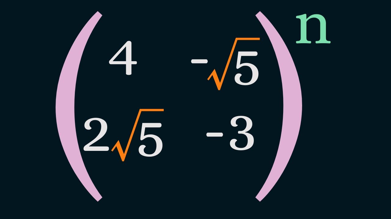










Eigenvalues and eigenvectors are fundamental concepts in linear algebra where an eigenvector x of a square matrix A satisfies Ax = λx, with λ being the corresponding eigenvalue; to find them, one solves the characteristic equation det(A - λI) = 0 to obtain eigenvalues, then substitutes each eigenvalue back into (A - λI)x = 0 and solves the resulting system to find the associated eigenvectors, noting that any scalar multiple of an eigenvector is also an eigenvector.
How to Find Eigenvalues and Eigenvectors | Linear Algebra
Added:Understanding of basic matrix operations, specifically matrix-vector multiplication and the identity matrix.
Ability to calculate the determinant of 2x2 and 3x3 square matrices.
Proficiency in solving systems of linear equations and finding the null space (kernel) of a matrix via row reduction.
Familiarity with basic algebraic concepts, particularly finding the roots of polynomial equations.
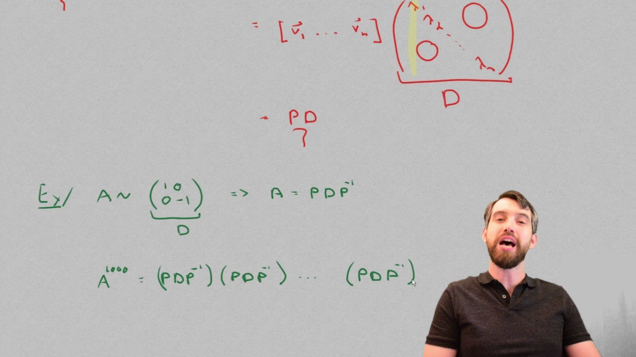
Matrix diagonalization and learning how to compute high powers of matrices efficiently.
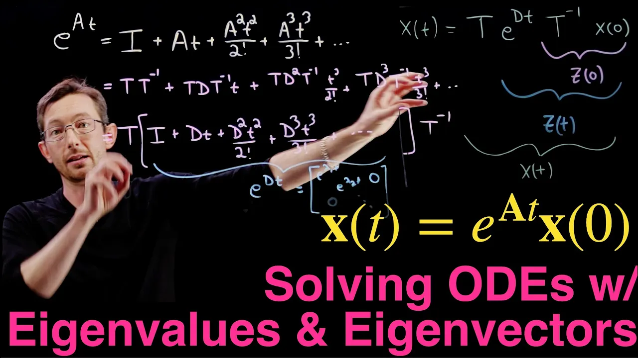
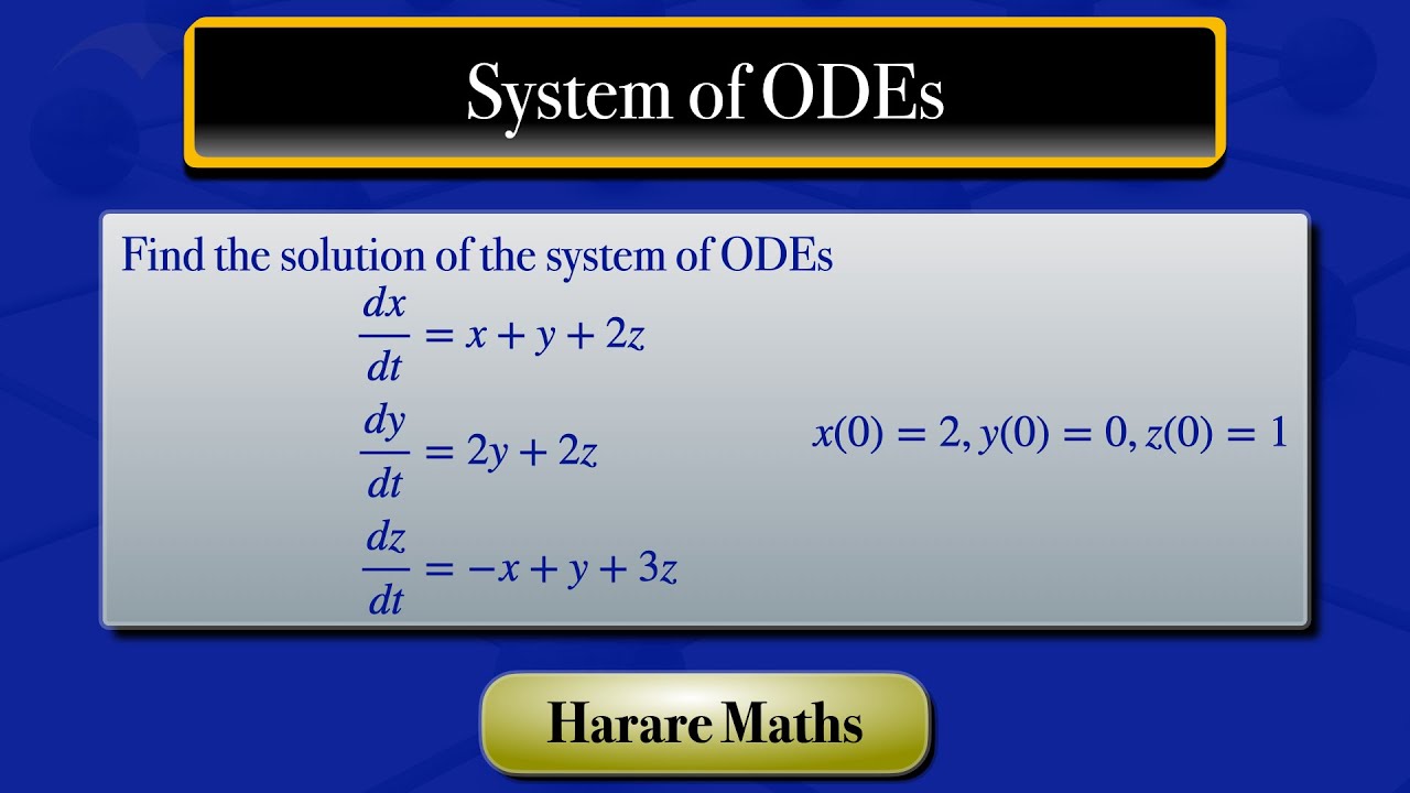
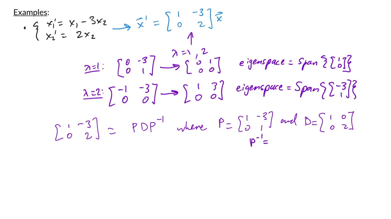
Applying eigenvalues and eigenvectors to solve systems of linear ordinary differential equations.
Exploring advanced matrix decompositions, such as the Spectral Theorem and Singular Value Decomposition (SVD).
Investigating practical applications like Principal Component Analysis (PCA) in data science and finding normal modes in physics.
1.2M views23.5Klikes17:09Original Release: 2019-07-17
It’s Professor Dave, I wanna tell you about eigenvalues and eigenvectors.
Eigenvalues and eigenvectors represent an incredibly useful concept in linear algebra, and we can see their application not just in math, but also in physics, especially quantum physics, which we have begun to learn about in the modern physics series.
Eigenvalues can be used to solve systems of linear differential equations, describe natural frequencies of vibrations, separate modes of motion, distinguish states of energy, and much more.
So just what are they exactly?
Let’s say we have matrix A, a square, n by n, matrix.
Eigenvectors are vectors that have a special relationship with matrix A, such that when you multiply A times the eigenvector x, you get back that same vector, multiplied by a scalar, lambda.
These scalars are called eigenvalues, or sometimes characteristic values.
In addition, these eigenvectors must be nontrivial, meaning that they are not just the zero vector.
The matrix A can have multiple eigenvalues, but no more than n, the number of rows and columns in the matrix.
Furthermore, each eigenvalue will have its own eigenvector that is associated with it.
Before we start trying to solve for eigenvalues or eigenvectors, let’s see them in action, so that we can further cement the definition we just mentioned.
Let’s say that matrix A is a 2 by 2 matrix with elements -3, 1, -2, and 0.
Now let’s check that the vector x = (1, 1) is an eigenvector.
To do this, we will simply multiply A by x and see if we get back x multiplied by some scalar.
Performing the multiplication, we get (-3 times 1 + 1 times 1, -2 times 1 + zero times 1), or (-3 + 1, -2 + 0), which simplifies to (-2, -2).
We can simply factor out a -2 from this and get -2 times (1, 1), which is just our original vector multiplied by -2.
We have not only verified that (1, 1) is in fact an eigenvector of our matrix, but also discovered that -2 is one of its eigenvalues.
Now that we are better acquainted with eigenvalues and eigenvectors, let’s start learning how to solve for them.
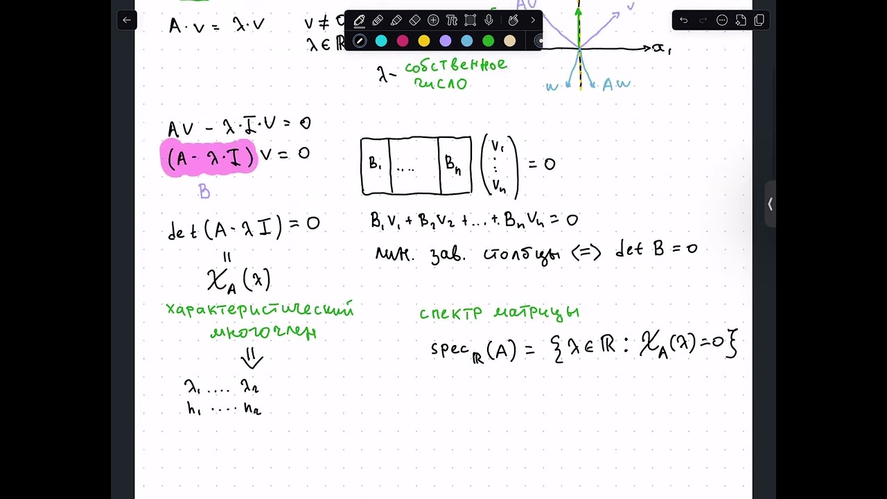
We know that the eigenvalues and eigenvectors of a square matrix, A, obey the equation Ax = λx.
In order to solve this, we will first subtract λx from both sides.
Then, in between lambda and x, we will insert the identity matrix, I, which is the matrix equivalent of multiplying by one, so we are not changing the equation by doing this.
Now we have Ax – λIx = the zero vector.
If we factor out the vector, we can rewrite this as the quantity (A - λI) times x = the zero vector.
Now we want nontrivial solutions to this equation, meaning that x can’t be the zero vector.
Let’s see what this means for (A - λI).
If this matrix were invertible, then we could multiply both sides by (A - λI) inverse, and get x = (A - λI) inverse times the zero vector, which would mean that x is zero.
To avoid this situation, (A - λI) can’t be invertible, and therefore, as we recall from learning about inverse matrices, the determinant of this matrix must be zero.
The determinant of A - λI will form a polynomial in λ often referred to as the “characteristic polynomial”, and the equation formed when the determinant equals zero is called the “characteristic equation”.
The solutions to this equation will be our eigenvalues.
Let’s try a concrete example so that this will make more sense.
Consider matrix A, which equals 1, 1; 4, 1.
We will take this matrix and subtract λI, where I is the two by two matrix with ones on the main diagonal and zeros for the other two entries.
Multiplying by lambda, we simply end up with lambdas on the main diagonal, and so in performing the subtraction, we will simply end up subtracting lambda from the main diagonal of A. That gives us 1 - λ, 1, 4, 1 - λ.
Now we must take the determinant of this matrix and set it equal to zero.
The determinant will be (1 – lambda times 1 – lambda) - the quantity (4 times 1).
Foiling out this first term leaves us with 1 - 2λ + λ2 - 4.
If we simplify and then set this equal to zero, that will give us a characteristic equation of λ2 - 2λ – 3 = 0.
If we recall our basic algebra, we can easily factor this, rewriting it as (λ - 3)(λ + 1) = 0.
This means that we have two solutions, 3 and -1.
These are the eigenvalues.
So to summarize what we just did, we found the determinant of A – λI and set it equal to zero, which was our characteristic equation, and then solving that equation gave us a pair of eigenvalues.
Once we have found the eigenvalues for a matrix, we can start solving for the eigenvectors.
This takes a bit more effort, and it must be done for each eigenvalue separately.
We will once again start the process by examining the A - λI part of (A - λI) times x = the zero vector.
This time we will actually plug in one of the eigenvalues we found for lambda and get a new matrix.
This new matrix, multiplied by our unknown vector x, equals zero, so in essence what we are left with is a system of equations that we can solve by any method we’ve learned so far.
The most consistent method here is to use row operations to get the matrix into row echelon form.
There will be times when we must “choose” values for the components of the eigenvectors, but it doesn’t really matter what we choose, because the solution we find by doing so only represents the form of eigenvectors.
Any scalar multiple of the vector we find through this method will also be an eigenvector.
We can easily demonstrate this as follows.
Assume the vector x is an eigenvector of A, so Ax = λx.
Now if we consider the vector cx, where c is a scalar, then A times this new vector can also be written as c times Ax since c is just a scalar.
We already know Ax = λx so this becomes cλx which can be rewritten as λ(cx).
So we get A(cx) = λ(cx) which makes the vector cx an eigenvector, by definition.
To make this process of solving for eigenvectors a little more clear, let’s once again consider the matrix A equals 1, 1; 4, 1.
We have already found the eigenvalues of this matrix to be 3 and -1, so let’s use these to find the related eigenvectors.
We can start with λ = 3 and plug this into A - λI.
We end up getting threes on this main diagonal, which means we will be subtracting 3 from the diagonal elements of A, leaving us with -2, 1, 4, -2.
Now once we have this, we will have to use row operations to get this in row echelon form.
In this case, we can simply add two times the first row to the second row, to get a new second row.
This turns the second row into zeros, and we are left with -2 and 1 in the first row.
Recall that we are solving the matrix equation (A - λI)x = 0, so this matrix multiplied by x equals zero.
Writing x as (x1, x2) and doing matrix multiplication, we end up with the equation -2x1 + x2 = 0.
Moving 2x1 to the other side, that leaves us with x2 = 2x1.
Let’s now “choose” x1 to be equal to 1, which makes x2 equal to 2.
So for the eigenvalue λ = 3, we get the eigenvector x = (1, 2).
However, recall that this vector only represents the form eigenvectors take for this eigenvalue.
We can have any multiple of this vector, and it will still be an eigenvector.
To put it simply, any vector where the second element is twice the first, will be an eigenvector.
Now let’s do the same thing for λ = -1.
We once again go back to A - λI, this time plugging in -1 for lambda.
In this case, by subtracting negative 1 from the main diagonal of A, we find the result to be 2, 1, 4, 2.
For our row operation this time, we will subtract two times the first row from the second row to get a new second row.
We are left with 2 and 1 in the first row, which this time makes our equation 2x1 + x2 = 0.
Moving x1 to the other side we are left with x2 = -2x1.
Keeping it simple, let’s again choose 1 for x1, and we get x2 = -2, making our vector x = (1, -2).
Again, any multiple of this vector will also qualify.
So the eigenvectors for λ = -1 are vectors with their second element being equal to -2 times the first element.
Now that we’ve gotten our feet wet, let’s go through one more example to really make sure we understand this process.
This time let’s take our matrix A to be 1, 0, 0; 3, -2, 0; 2, 3, 4 and for this we will find the eigenvalues and eigenvectors.
First, to find the eigenvalues, let’s find A - λI, which will mean subtracting lambda from the terms in the main diagonal of A. Then we will take the determinant of this new matrix, and set the polynomial equal to zero.
Thanks to the form of our matrix, with two zeros in the top row, the determinant of A - λI is relatively simple.
We get (1 - λ) times [(-2 - λ)(4 - λ) – (0 times 3)], then minus zero, and then plus zero.
This simplifies to the product of these three binomials, and setting this equal to zero, we end up with a characteristic equation that is already completely factored.
(1 - λ)(-2 - λ)(4 - λ) = 0.
So our solutions are λ = 1, λ = -2, and λ = 4, and these are the eigenvalues for this matrix.
Now that we have the eigenvalues, we can solve for the eigenvectors that are related to each of them.
Let’s start with λ = 1.
We will go back to our matrix given by A – λI, and plugging in λ = 1, we will subtract 1 from the terms in the main diagonal to get the matrix 0, 0, 0; 3, -3, 0; 2, 3, 3.
We could go through row operations from here, but the form of our matrix in this case makes it simple to solve if we jump right into equation form.
The top row gives no information, but the second row tells us 3x1 - 3x2 = 0.
Solving this we see that x1 = x2, and for this case let’s choose x2 to be 1.
So both x1 and x2 are therefore equal to one.
The final row tells us that 2x1 + 3x2 + 3x3 = 0, but we’ve already chosen x1 and x2 to be equal to 1, so plugging those values in, we get 2 + 3 + 3x3 = 0.
We end up getting x3 = -5/3, making our eigenvectors any multiple of (1, 1, -5/3).
Next we will find the eigenvectors for λ = -2.
Plugging this value into A – λI, we subtract -2 from the main diagonal to get 3, 0, 0; 3, 0, 0; 2, 3, 6.
Expressing this in equation form, the first row tells us that 3x1 = 0, so x1 must be zero.
The second row tells us the same thing.
Meanwhile, the final row becomes 2x1 + 3x2 + 6x3 = 0.
We already know that x1 is 0, so we are left with 3x2 + 6x3 = 0, or x2 = -2x3.
We will now choose x3 to be 1, making x2 = -2.
So the eigenvectors have the form (0, -2, 1).
And finally let’s do the third eigenvalue λ = 4.
The matrix A - λI requires subtracting 4 from the main diagonal, so this becomes -3, 0, 0; 3, -6, 0; 2, 3, 0.
The first row tells us that -3x1 = 0, so once again x1 is zero.
The second row tells us 3x1 - 6x2 = 0, but since x1 is 0, we are left with -6x2 = 0.
So x2 must also be zero.
The third row becomes 2x1 - 3x2 = 0.
We already know that both x1 and x2 are zero, but we have no information about x3.
This makes x3 a free variable.
In this case we can just choose 1, making our eigenvectors have the form (0, 0, 1).
Now that we have sufficiently discussed the important process of finding eigenvalues and eigenvectors, let’s check comprehension.
Up Next

9:33
Gradient Vector in Multivariable Calculus: Definition & Examples
@mathemation
1.9K views•2021-04-07

4:43
Elliptic Curve Cryptography Explained: ECC, ECDSA, ECDH
@PracticalNetworking
28.5K views•2024-10-21
5:53
Divisibility, Prime Numbers, & Prime Factorization | Math Basics
@ProfessorDaveExplains
158.6K views•2017-08-20

6:00
The Mathematical Impossibility of Accurate World Maps
@Vox
23.3M views•2016-12-02
Related Study Plans & Knowledge Roadmaps
Structured learning paths in Mathematics
mathematics
Tensor Calculus: Vectors to Riemann Curvature
01Mathematical Foundations: Linear Algebra & Calculus
02Covectors, Dual Spaces, and Tensor Basics
03The Metric Tensor and Index Gymnastics
+ 2 more learning modules
40h5 modules
Explore Roadmap
mathematics
Gödel's Incompleteness: Logic, Proofs & Limits
01Introduction to Formal Systems & Hilbert's Dream
02Set Theory, Cardinality, and Cantor's Diagonal Argument
03Arithmetization and Gödel Numbering
+ 2 more learning modules
14h5 modules
Explore Roadmap
mathematics
Galois Theory: Fields, Groups & Solvability
01Foundations of Abstract Algebra: Groups & Fields
02Polynomials & Field Extensions
03Splitting Fields & Symmetries
+ 2 more learning modules
24h5 modules
Explore Roadmap
mathematics
Non-Euclidean Geometry: Models & Geodesics
01Euclid's Fifth Postulate and the Birth of New Geometries
02Hyperbolic Space and the Poincaré Disk Model
03Geodesics: Defining Straight Lines in Curved Spaces
+ 2 more learning modules
15h5 modules
Explore Roadmap