

















![Test for Conservative Vector Field [Dr. Scott Adamson]](https://i.ytimg.com/vi/Ao86ANLPd5c/maxresdefault.jpg)

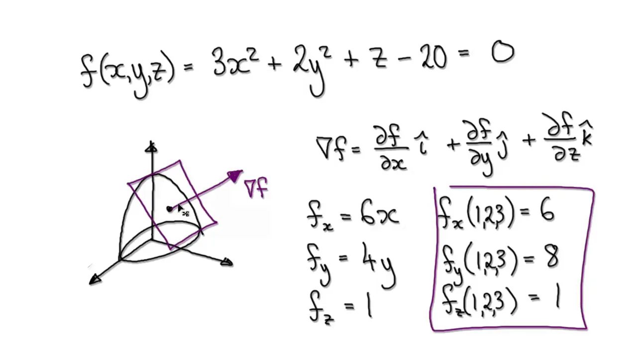
The gradient vector ∇f(x,y) = [f_x(x,y), f_y(x,y)] is a vector-valued function that bundles the partial derivatives of a multivariable function into a single vector, which simplifies many formulas in multivariable calculus including directional derivatives (∇f·u), linear approximations (f(a) + ∇f·(x-a)), and the chain rule for paths (∇f(r(t))·r'(t)). The gradient vector plays the role of the derivative in single-variable calculus, appearing in analogous positions in multivariable formulas.
Gradient Vector in Multivariable Calculus: Definition & Examples
Added:Understanding of partial derivatives and how to compute them for functions of multiple variables.
Basic vector algebra, including vector representation, magnitude, and the algebraic definition of the dot product.
Familiarity with functions of several variables and visualizing their graphs as multi-dimensional surfaces.
The conceptual foundation of a derivative as a rate of change from single-variable calculus.
Geometric interpretations of the gradient, specifically its relation to the direction of steepest ascent and its orthogonality to level curves and surfaces.
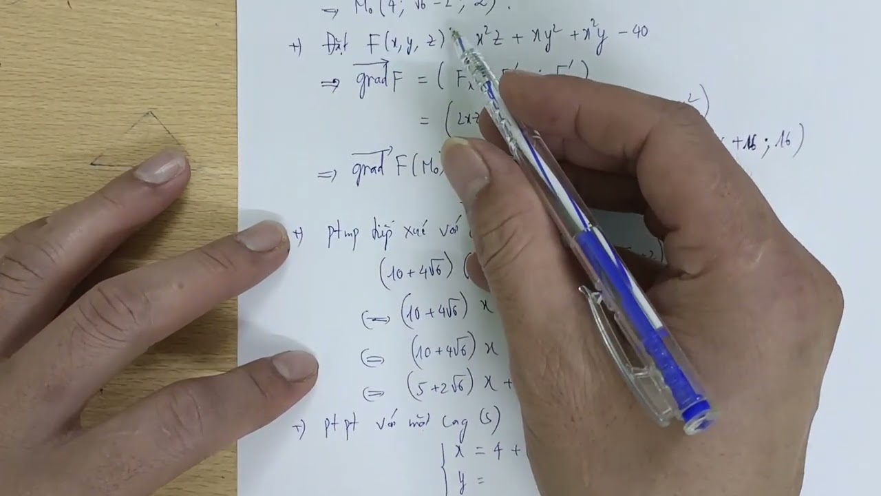
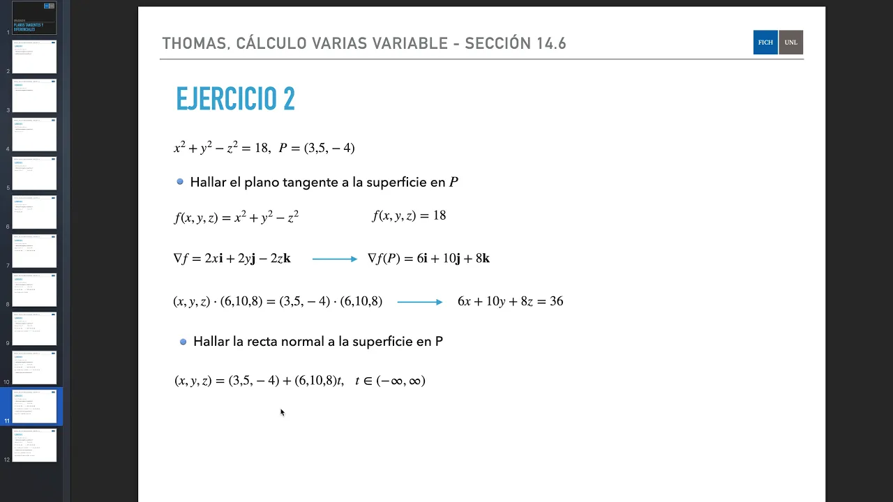
Finding the equations of tangent planes and normal lines to surfaces using the gradient vector.
Optimization of multivariable functions, including finding local extrema and utilizing Lagrange Multipliers for constrained optimization.
The study of conservative vector fields and the Fundamental Theorem of Line Integrals, where the gradient vector field plays a central role.
1.9K views25likes9:33Original Release: 2021-04-07
hey there folks and welcome back in our last lesson we introduced the notion of a directional derivative this was sort of like a partial derivative right it measures a rate of change of our function but now we're no longer restricted to just moving in the x or y directions starting at a point a b we can measure the rate of change in any direction by moving with some unit vector u to calculate directional derivatives we can use the following amazing formula that we derived in our overview video it says that a directional derivative is really a combination of our two partial derivatives and the entries of our unit vector u now i think this formula looks pretty cute already but it turns out we can make it even cuter and more compact by bundling these two partial derivatives together as a single vector that's exactly what we're going to do we're going to group them together as entries of a vector f x a b f y a b you may notice that our directional derivative formula is then given by the dot product of this vector of partial derivatives with the vector u1 u2 pretty simple right it turns out there are lots of formulas in multi-variable calculus where the same kind of trick can be applied the two partial derivatives f x and f y appear together and the formula can be simplified by bundling them into a single vector can you think of any examples like this that we've seen so far we'll talk about that in just a moment for now trust me when i say that this vector appears pretty often in multi-variable calculus often enough that it deserves its own name we're going to call it the gradient vector of our function f so specifically if i have a function f from r 2 to r we are going to define its gradient vector evaluated at the point x y by this symbol this upside down triangle nabla f or del f at x y and it's the vector of partial derivatives f x x y f y x y now there's nothing special here about r two we could have made this exact same definition with a function that starts in r n uh we would just have to add more components so for example if f starts from r 3 and maps into r its gradient is the vector f x f y f z using this new notation for our gradient we can write our directional derivative formula very compactly as del f at a b dot u vector pretty nice huh very simple and very easy to remember let's check out some other formulas that we've seen so far that can be simplified using the gradient vector in addition to our directional derivative formula our two partial derivatives appear together in our tangent plane linear approximation formula so maybe we can simplify this using the gradient vector what we have here is f of a b plus another dot product like expression right this is the dot product of the vector f x a b f y a b that looks like our gradient with the vector x minus a y minus b now to make this look a little bit more familiar what i'm going to do is bundle the x and y terms together in a single vector which i'm going to call x as well so x vector is the vector x y and i'm going to do the same thing for a and b i'll define a vector to be the vector a b i can therefore rewrite my equation as f of a plus del f at a b dot x vector minus a vector does this equation look somewhat familiar it should this looks a lot like the equation of a tangent line that you would have known back in calc one remember the equation of the tangent line at x equals a is l of x equals f of a plus f prime a times x minus a that looks very similar to what we have here except now it looks like our gradient vector is playing the role of the derivative that you used back in calc 1.
we can do something similar with the chain rule for paths once again our partial derivatives are appearing together as a quick reminder the chain rule for paths is used when we're trying to take the derivative of a function defined along a parametric curve so maybe our parametric equation here is r of t r of t equals x of t y of t what we have is a dot product expression it's the dot product of f x at x y f y at x y with the vector d x over d t d y over dt ah but notice this is exactly the gradient of f applied to r of t right we need an x y in here and now we're taking the dot product with r prime t okay folks this is starting to get a little eerie this expression here looks almost identical to the chain rule that you would have known back in calc 1.
the chain rule from calc 1 says that the derivative of f of g of t is f prime g of t times g prime t here we have del f of r of t dot r prime t once again it looks like my gradient vector is playing the role of a derivative this is a real theme in multivariable calculus you'll often see the gradient vector showing up in places where the derivative used to appear now let's check out some examples okay we've seen how gradient vectors appear in some of our familiar formulas but we haven't actually computed any gradient vectors so let's try a couple examples here i want to compute the gradient vector for this function f of x y equals 8 minus x squared over 2 minus y squared over 2.
by definition my gradient is the vector of partial derivatives so i'll start by taking the partial with respect to x i get minus two x over two and the partial with respect to y is similarly minus two y over two cancel the twos that leaves us with a vector minus x minus y that's our gradient at the point x y we can do the exact same thing with this function except now i think we'll probably need the chain rule when i take the partial with respect to x i do the derivative of the inside to get 2x but when i take the derivative of the square root function i get 1 over 2 times the square root of now i leave the inside alone x squared plus y squared similarly my partial derivative with respect to y is 2y divided by 2 times the square root of x squared plus y squared once again we cancel some twos and we're left with the vector x over the square root of x squared plus y squared y over the square root of x squared plus y squared now i know what you're thinking ah come on zach this is easy we're just finding partial derivatives and then plopping them into a vector yeah i agree finding the partial derivatives and building the gradient vector isn't too hard but there's a bit more going on in these examples that i want to point out based on how we've written this expression here it looks like the gradient vector is sort of like a function right it's taking in two inputs x and y and it's spitting out a vector output this means that at every point x y in my 2d plane i can plot this gradient vector del f at x y when you plot these vectors alongside the graph of your function you get some really interesting information so let's try plotting a few of these vectors in our first example if we consider the gradient at the point 1 0 which is somewhere over here well that's the vector minus 1 0 it points us in this direction likewise if we consider the gradient at the vector 0 1 we get the vector 0 minus 1.
it points us in this direction notice that both of these gradient vectors are pointing us back toward the origin in this example i think that's always going to be the case after all if you give me a point x y then the gradient minus x minus y is going to point me back from where i started it's going to point me back to 0 0. now that's a really interesting feature after all this is a vector of partial derivatives why should we believe that they're going to be pointing us back toward the origin what's special about this function that would cause all of these arrows to point us in that direction i wonder do you think the same behavior is going to happen with this function let's plot a few gradients and find out in this example del f at 1 0 is going to give me the vector 1 over the square root of 1 squared plus 0 squared that's 1 and 0 over this square root that's 0.
so at 1 0 i get the vector 1 0.
del f at 0 1 is going to give me 0 in the first component and then 1 in the second component so my gradient here is going to be pointing in this direction notice now my gradients are pointing away from the origin and i'll let you convince yourself that that's going to be the case at all points in this 2d plane so why is it that the gradients point us toward the origin in this example and away from the origin here it turns out that there's a very deep and intimate connection between our gradient vector and our directional derivatives and it's that connection that helps to explain this unusual behavior we're going to learn more about this in our next lesson
Up Next

6:54
Visualizing Partial Derivatives: f(x,y)=x^2*y at (2,3)
@MathTeacher80031
468 views•2022-09-07

4:43
Elliptic Curve Cryptography Explained: ECC, ECDSA, ECDH
@PracticalNetworking
28.5K views•2024-10-21

10:44
Fourier Series Introduction: The Big Idea Explained
@DrTrefor
387K views•2021-05-03

6:00
The Mathematical Impossibility of Accurate World Maps
@Vox
23.3M views•2016-12-02
Related Study Plans & Knowledge Roadmaps
Structured learning paths in Mathematics
mathematics
Tensor Calculus: Vectors to Riemann Curvature
01Mathematical Foundations: Linear Algebra & Calculus
02Covectors, Dual Spaces, and Tensor Basics
03The Metric Tensor and Index Gymnastics
+ 2 more learning modules
40h5 modules
Explore Roadmap
mathematics
Gödel's Incompleteness: Logic, Proofs & Limits
01Introduction to Formal Systems & Hilbert's Dream
02Set Theory, Cardinality, and Cantor's Diagonal Argument
03Arithmetization and Gödel Numbering
+ 2 more learning modules
14h5 modules
Explore Roadmap
mathematics
Galois Theory: Fields, Groups & Solvability
01Foundations of Abstract Algebra: Groups & Fields
02Polynomials & Field Extensions
03Splitting Fields & Symmetries
+ 2 more learning modules
24h5 modules
Explore Roadmap
mathematics
Non-Euclidean Geometry: Models & Geodesics
01Euclid's Fifth Postulate and the Birth of New Geometries
02Hyperbolic Space and the Poincaré Disk Model
03Geodesics: Defining Straight Lines in Curved Spaces
+ 2 more learning modules
15h5 modules
Explore Roadmap