This tutorial demonstrates how to build a raw EMG (Electromyography) signal rectifier by capturing raw EMG signals with Arduino and processing them in MATLAB, where the rectifier converts the raw EMG signals into a usable format for muscle activity analysis.
EMG Signal Rectification with MATLAB and Arduino: A Step-by-Step Demo
Added:Deep Dive
Basic understanding of Electromyography (EMG) physiology, including how skeletal muscle contractions generate detectable biopotential signals.

Basics of Electromyography
5.1K
Electromyography (EMG) measures the electrical activity of muscles by recording motor unit action potentials generated when motor neurons activate muscle fibers; the process involves understanding motor units (comprising motor neurons and their innervated muscle fibers), the neuromuscular junction where action potentials trigger muscle contraction through calcium release, and the biophysics of signal generation including volume conduction and crosstalk effects, with EMG instrumentation utilizing electrodes (surface, needle, or array types), amplifiers, and recording systems to capture and interpret these electrical signals for diagnostic purposes.
Click to watch →

Simple Muscle twitch & EMG ( Physiology Practical )
690
Electromyography (EMG) records electrical activity in skeletal muscles using electrodes: intramuscular (inserted into muscle) and surface (placed on skin). The recording (electromyogram) shows muscle electrical activity over time. At rest, muscles show small resting potential due to continuous tonus. As contraction intensity increases, more motor units are recruited, producing larger signals. At strong contraction, an interference pattern appears due to overlapping signals from multiple motor units. EMG is used to diagnose neurological and muscular disorders by identifying where problems occur in the neuromuscular system.
Click to watch →
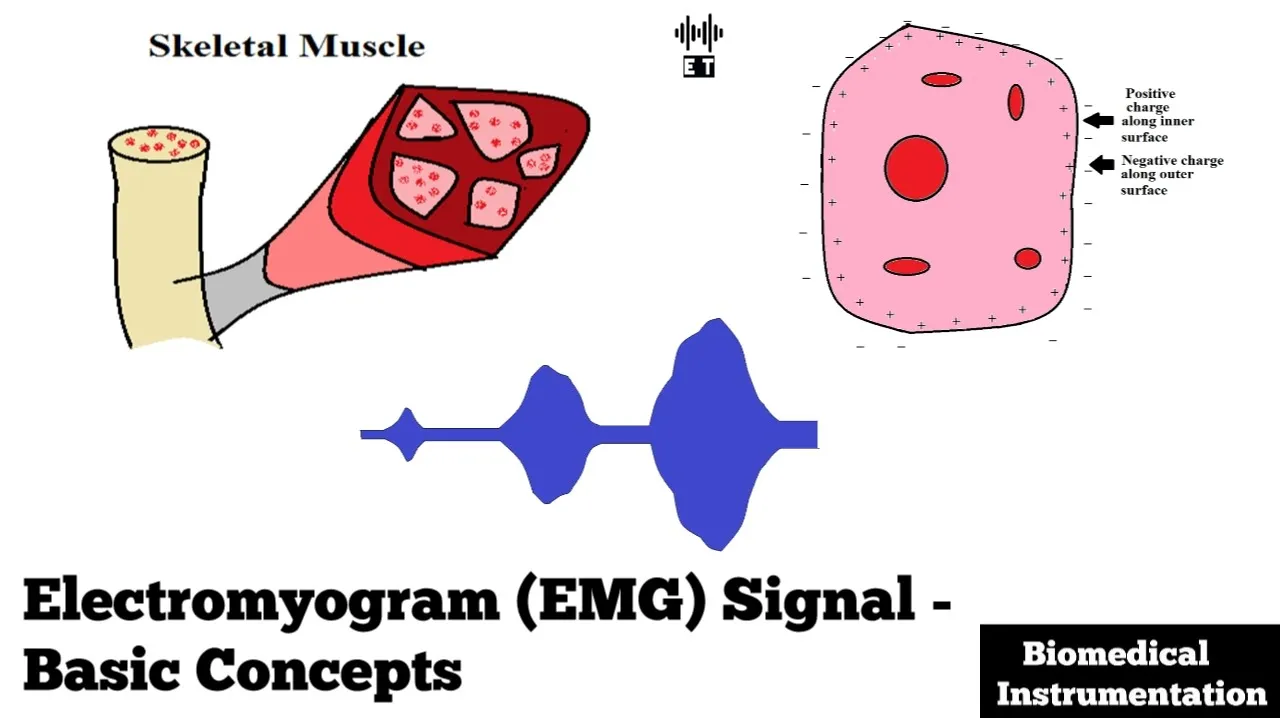
Electromyogram (EMG) Signal | Basic Concepts | Biomedical Instrumentation
9.9K
An electromyogram (EMG) is the recording of electrical activity generated by skeletal muscle contractions, with an amplitude range of 0.1 to 5 microvolts and frequency range of 5 Hz to 2 kHz; it follows the same cellular mechanism as ECG and EEG, where muscle cells transition from a resting state (negative inner surface, positive outer surface at approximately -90 mV) to an excited state during contraction, producing an action potential called depolarization, followed by repolarization to return to the resting potential.
Click to watch →
EMG--concepts to understand before lab -- Electromyography -- Muscle Physiology Lab
20.7K
Electromyography (EMG) measures electrical activity produced by muscles during contraction. The underlying theory connects EMG readings to motor unit recruitment, explaining how muscles generate varying force. Muscle cells maintain a resting membrane potential with negative interior charge. When stimulated, this charge rapidly reverses (action potential), triggering contraction. This charge reversal returns almost immediately. Graphically, resting potential shows a stable negative baseline, while action potentials appear as characteristic spikes. Each spike corresponds to one muscle cell contraction, establishing the direct relationship between electrical events and mechanical output in muscle physiology.
Click to watch →

Electromyogram EMG Lec4 Biophysics I
6.3K
Electromyography (EMG) is a diagnostic technique that measures electrical signals produced by muscles during contraction. When muscles contract, they generate electrical signals that can be detected and recorded. The EMG device consists of electrodes placed on the muscle that capture these signals and display them on a screen. Muscle contraction is triggered by action potentials (electrical signals) that travel from motor neurons to the muscle through the neuromuscular junction. This allows assessment of whether muscles are functioning properly by measuring their electrical activities.
Click to watch →
Deep Dive
Fundamentals of Arduino hardware operation, specifically analog-to-digital conversion (ADC) and configuring serial communication rates.
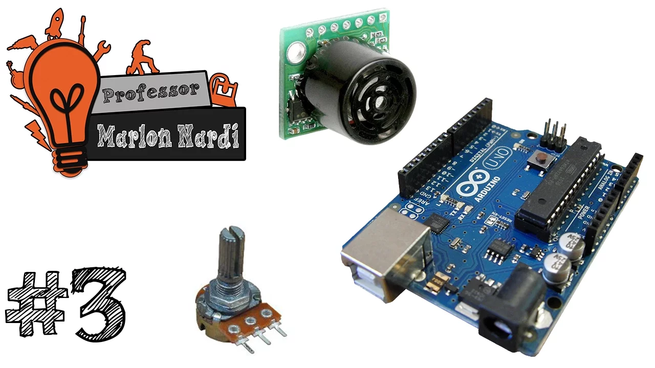
Curso de Arduino #3 | Entradas analógicas, Conversor AD, Pino Aref, Variáveis, SM
29.9K
This comprehensive section covers the complete theory and practice of analog-to-digital conversion in Arduino. Analog signals are continuous with infinite amplitude values, while digital signals are discrete with only two states (0 or 1). The ADC standardizes analog signals into digital format that microcontrollers can process. The Arduino Mega has 16 analog inputs with 10-bit resolution, producing 1024 values (0-1023) from 0-5V input. Each ADC unit represents approximately 4.9mV. Variables are memory positions storing data for program logic, with 'int' (2 bytes, -32,768 to 32,767) and 'float' (4 bytes, decimal values) being the most common types. The analogRead() function reads analog values and returns 0-1023. Practical applications include using potentiometers as voltage dividers to simulate 0-5V signals, controlling LED timing based on input values, and creating voltmeters by calculating voltage from ADC values.
Click to watch →
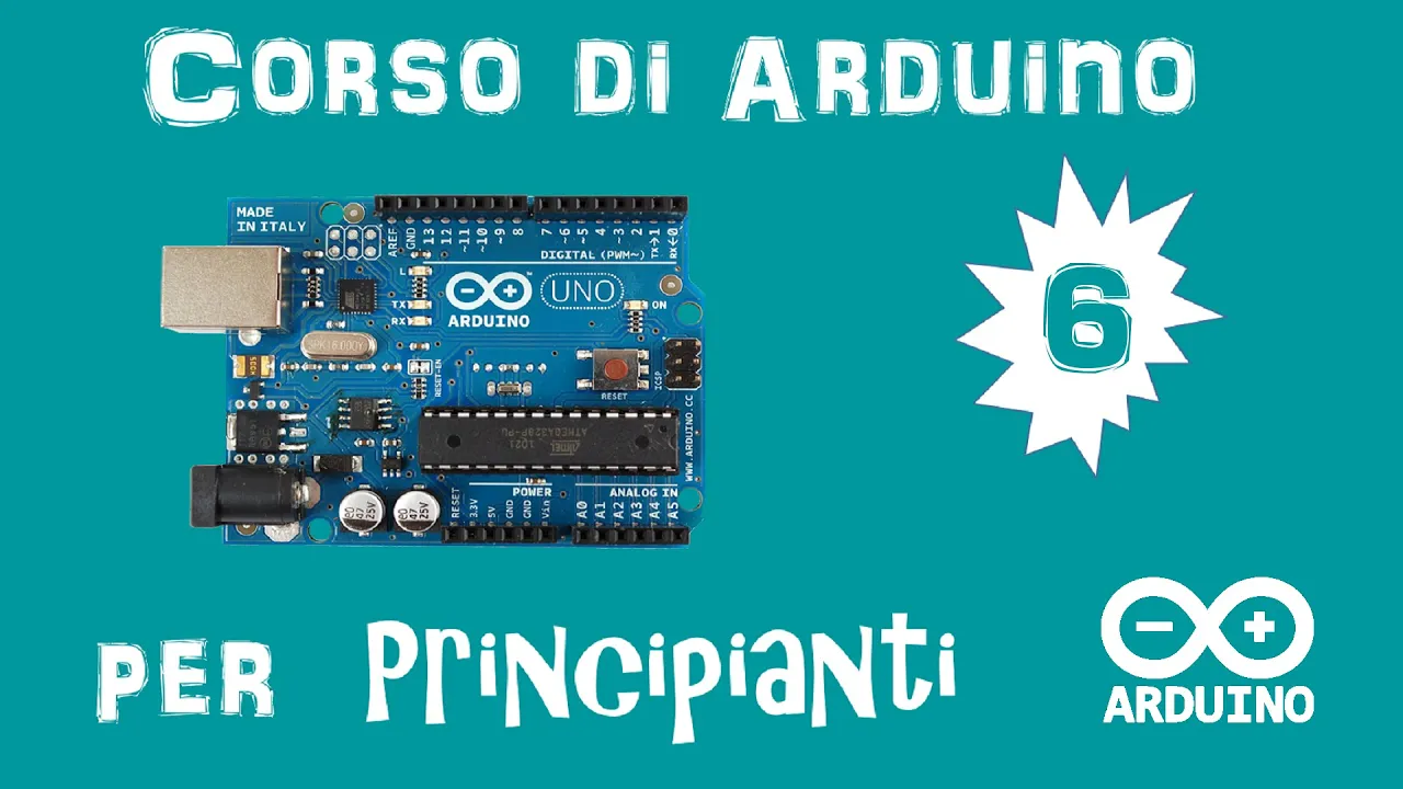
Arduino Tutorial ITA #6: Comunicazione seriale
90.4K
Serial communication is a digital method that transmits data one bit at a time in sequence, requiring only one cable (such as USB) for device-to-device communication. In Arduino, serial communication must be initialized in the setup() function using Serial.begin(baudRate), where baud rate determines transmission speed. A baud rate of 9600 means 9,600 characters per second, which is standard for Arduino projects despite being slow for modern electronics. Basic output is achieved using Serial.println() with characters in double quotes, and the function automatically adds a newline character for readable multi-line output.
Click to watch →

31. Arduino for Production! How to use the ADC with Interrupts
103.1K
This section explains how to configure the ADC hardware including pin selection, reference voltage configuration, and timing parameters. The ADC uses a multiplexer (MUX) controlled via ADMUX register bits to select input channels. The reference voltage determines the measurement range and is configured through REFS bits. The pre-scaler divides the system clock to achieve the required 50-200 kHz input frequency range for proper ADC operation. These configurations must be done before enabling the ADC to ensure correct operation.
Click to watch →

#340 How good are the ADCs inside Arduinos, ESP8266, and ESP32? And external ADCs (ADS1115)
215.6K
ADCs convert analog voltages to digital numbers, enabling microcontrollers to process real-world signals. Two main architectures exist: parallel comparator ADCs (fast, high-speed applications up to GHz, but poor scalability requiring 2^n comparators for n-bit resolution) and successive approximation ADCs (slower but more practical with single comparator and integrated DAC). Resolution defines step size (reference/2^n), while accuracy depends on component precision. These concepts form the foundation for understanding all subsequent ADC discussions.
Click to watch →

Curso de Arduino #10 - Portas analógicas
21K
For successful serial communication, the baud rate configured in the Arduino code must exactly match the baud rate setting in the Serial Monitor software. If the baud rates differ, communication errors occur and the displayed data becomes garbled or unreadable. The Arduino IDE allows you to change the baud rate in the Serial Monitor settings, but it must match the code's Serial.begin() parameter.
Click to watch →
Deep Dive
Core concepts of signal processing, such as raw signal amplitude, frequency, and the mathematical difference between alternating (AC) and direct (DC) components.

Basic Electrical and Electronics Engineering KTU 2024 Scheme Group C & D | BEE Module 1 Part 2
1.2K
Direct Current (DC) maintains constant magnitude regardless of time, while Alternating Current (AC) varies periodically with time. DC sources include cells and batteries, producing steady signals. AC sources are generators producing fluctuating signals. The major difference is that DC signals remain constant while AC signals change amplitude and direction periodically. AC signals are represented mathematically as x(t) = EM sin(ωt + φ), where EM is the peak value, ω is angular frequency, and φ is the phase angle.
Click to watch →

Fundamentals of AC Signals
10.5K
AC (Alternating Current) signals change magnitude and polarity at regular intervals, while DC (Direct Current) signals maintain constant amplitude and direction. AC signals are safer for long-distance transmission with minimal power loss, can change direction during flow, and have variable frequency depending on the country. DC signals have zero frequency and can only work with resistive loads. The sine wave voltage equation is V = Vm sin(ωt), where Vm is maximum amplitude, ω is angular frequency (2π/T), and t is time. Key parameters include: Cycle (one complete set of positive and negative values), Time Period (time for one complete cycle), Frequency (cycles per unit time, f = 1/T), Amplitude (maximum value), Phase Angle (angular displacement from zero degrees), and Phase Difference (angular displacement between starting points of two waveforms). Phase lead occurs when waves start before the origin (+θ), while phase lag occurs when they start after (-φ).
Click to watch →
Что такое Спектр напряжения, Гармоники, Преобразование Фурье, FFT, THD - это просто!
43K
This section covers the basic parameters of electrical signals. AC signals alternate between positive and negative values, with amplitude being the peak voltage and RMS (effective) value being Vamplitude/√2. For example, 220V RMS corresponds to approximately 310V amplitude. DC signals maintain constant polarity without oscillation. The period is the time for one complete cycle, while frequency measures cycles per second (Hz). These fundamental concepts form the basis for understanding more complex signal analysis techniques.
Click to watch →

Circuits Electriques : (MPI) - Chapitre 1 : Signaux Electriques
1.4K
Electrical signals are classified into three main types: (1) Analog signals vary continuously over time, such as microphone output; (2) Digital signals take discrete values (0 or 1), like those from logic gates; (3) Pulse Code Modulation (PCM) signals consist of multiple digital values representing information. Periodic signals repeat their pattern at regular intervals, with the period being the smallest time interval after which the pattern repeats exactly. Non-periodic signals do not repeat and have no repeating cycle. Amplitude represents the strength of a signal, calculated as the difference between maximum and minimum values. Peak-to-peak amplitude is the total range from maximum to minimum. Frequency measures how fast a signal repeats, calculated as the reciprocal of the period (Frequency = 1/Period). Duty cycle is the ratio of active time to total period, calculated as (Active Time / Total Period) × 100%. For discrete signals, average value is found by summing all values and dividing by the count. For continuous signals, average value is calculated by integrating the signal over a period and dividing by the period length. RMS (Root Mean Square) value represents the effective value of a signal, calculated by integrating the squared signal over a period, dividing by the period, and taking the square root. Any signal can be decomposed into DC (average) and AC (alternating) components. The DC component is the average value, found by dividing the total area under the curve by the period. The AC component is found by subtracting the DC component from the original signal. The AC component has an average value of zero and represents the varying part of the signal.
Click to watch →

25.AC Fundamentals @ganapathireddy
415
AC analysis is more complex than DC analysis because AC signals contain multiple parameters that must be understood: peak value, peak-to-peak value, time, time period, frequency, average value, RMS value, form factor, and peak factor. For DC signals, capacitors act as open circuits and inductors as short circuits, but for AC signals, concepts like reactance, impedance, phasor, and power factor become essential. Any signal is characterized by three fundamental parameters: amplitude (peak value), frequency (cycles per second), and phase (starting position). The general form is f(t) = A sin(ωt ± θ), where A is amplitude, ω is angular frequency, and θ is phase. Sine function is preferred over cosine because it starts from zero when t = 0.
Click to watch →
Deep Dive
Basic proficiency in MATLAB programming, including data visualization, variable manipulation, and writing scripts to handle array operations.
Matlab: Lecture 1
147.7K
MATLAB is a programming language for engineering and scientific applications. The interface includes the Command Window for typing code and viewing results, Workspace for storing variable values, and Command History for tracking executed commands. Basic arithmetic operations can be performed directly, with results automatically assigned to 'ans'. Variables can be named with letters, numbers, and underscores but cannot contain spaces. MATLAB is case-sensitive. To suppress output, use semicolons. M-files are text files that store code and can be executed as complete programs. Always start M-files with 'clear' and 'clc' for a clean workspace. File names cannot contain spaces or reserved words like 'matlab' or 'problem'. Comments use the percent sign (%) and are not executed as code. Arrays are created using colon notation: 'start:increment:end'. Element-wise operations require a dot before the operator (e.g., 't.^2'). The 'length' function returns array size, and array indexing uses 1-based indexing. Basic plots use 'plot(X, Y)'. Add titles and axis labels using 'title', 'xlabel', and 'ylabel' with single quotation marks. Multiple datasets can be plotted on the same figure using 'plot(X, Y1, X, Y2)'. Plot styles can be customized by adding a third argument to 'plot': 'o' for circles, '*' for asterisks, 'g' for green. The 'help plot' command provides available plot styles. For more comprehensive help, use the Help Browser. To get help on specific functions, type 'help function_name'. MATLAB handles complex numbers (a + bi) by typing them directly, such as 'z = 1 + 3i'. MATLAB automatically recognizes 'i' as the imaginary unit, and 'i*i' equals -1. Mathematical functions include 'exp' for exponential, 'sqrt' for square root, 'log' for natural logarithm, 'log10' for base-10 logarithm, 'cos' for cosine, 'sin' for sine, 'tan' for tangent, and 'pi' for π. MATLAB has different display formats: 'format short' (default) shows 4 decimal places, while 'format long' shows 15 decimal places. The actual stored values remain the same regardless of display format. 'format short' is recommended for homework assignments.
Click to watch →

Introduction to MATLAB
611
MATLAB is an interpreted programming environment for scientific computing. The interface includes a file browser, command window, workspace, and command history. Basic operations include calculator functionality where calculations produce variables automatically stored as 'ans'. Scripts are text files saved with '.m' extension for storing reusable commands. Variables are created using '=' (e.g., 't = 10'). Arrays use colon notation 'start:step:end' (e.g., 't = 1:10'). Random matrices use 'rand(m,n)'. The 'clc' command clears the command window, while 'clear' removes all variables. For plotting, use 'plot(x,y)' with 'xlabel', 'ylabel', 'grid', and 'hold on' for multiple curves. Functions can be created as anonymous functions using @ symbol (e.g., 'fn = @(t) sin(t) + cos(t)') or as separate function files. Complex numbers use 'i' or 'j' notation (e.g., 'a = 1 + 1i'). All operations work with complex numbers. Functions can accept arrays or matrices as inputs and return corresponding outputs, enabling vectorized operations without explicit loops.
Click to watch →
Pengenalan Coding MATLAB Untuk Pemula
421
MATLAB is a programming language for engineers and scientists used for mathematical modeling, numerical analysis, statistics, economics, and artificial intelligence. Basic operations use standard symbols: * for multiplication, / for division, + for addition. Variables are created with the equals sign (=) and can be reassigned. MATLAB is case-sensitive, treating 'x' and 'X' as different variables. Multiple variables can be assigned in one line using semicolons. Matrices are created using square brackets with elements separated by spaces or commas, and rows separated by semicolons. Matrix multiplication uses the * operator with compatible dimensions. Submatrices are extracted using row and column indices. Individual elements are accessed with matrix(row, column). The plot command creates 2D graphs by defining x and y values and using plot(x, y) to display relationships.
Click to watch →

Getting Started with MATLAB R2012b
89.2K
MATLAB is an array-based programming language where variables can be vectors, matrices, or n-dimensional arrays; basic operations include creating variables with square brackets, using the colon operator for equally spaced arrays, performing matrix operations like transpose and multiplication, and plotting data with commands such as plot() and surf().
Click to watch →

Prise en main de MATLAB_02
600
MATLAB distinguishes between scripts and functions. Scripts are sequences of instructions in .m files without input/output arguments, working directly in the workspace where all variables become global. Functions are specialized M-files with input/output arguments that interact with the workspace only through these variables, keeping other variables local. Scripts consist of three blocks: data acquisition, processing, and display. Functions use the syntax 'function [output] = function_name(input)' and can be called directly or through programs. The dot notation enables vectorized operations on matrices. MATLAB's visualization capabilities include 2D plotting with plot() and subplot() for dividing figures into multiple subplots, 3D plotting with plot3() for parametric curves, and image processing with image() for displaying pixelated images as matrices.
Click to watch →
Prerequisite Knowledge
- Concept 01Basic understanding of Electromyography (EMG) physiology, including how skeletal muscle contractions generate detectable biopotential signals.
- Concept 02Fundamentals of Arduino hardware operation, specifically analog-to-digital conversion (ADC) and configuring serial communication rates.
- Concept 03Core concepts of signal processing, such as raw signal amplitude, frequency, and the mathematical difference between alternating (AC) and direct (DC) components.
- Concept 04Basic proficiency in MATLAB programming, including data visualization, variable manipulation, and writing scripts to handle array operations.
Subsequent Learning
- Step 01Applying advanced digital filters, such as Butterworth bandpass and low-pass filters, to isolate the frequency bands of interest and reduce high-frequency noise.
- Step 02Implementing envelope detection algorithms, such as Root Mean Square (RMS) and moving average filters, to extract the smooth amplitude envelope of muscle activity.
- Step 03Extracting key EMG features in both time and frequency domains (e.g., Mean Absolute Value, Zero Crossings, Median Frequency) to analyze muscle fatigue.
- Step 04Designing real-time myoelectric control applications, such as using processed EMG signals to control robotic grippers, prosthetics, or video games.
Start
Acceptance
External
Connection
Audience
Start
0:46Playing Section
- 1
Initiates the core discussion.
- 2
Sets the stage for main content.
Limitations of Time-Domain Rectification and the Necessity of Time-Frequency Analysis
While signal rectification is a classic, computationally simple method for estimating muscle activation amplitude, it has significant limitations. Rectification is a non-linear process that discards the phase information of the raw electromyography (EMG) signal and alters its spectral characteristics, potentially introducing artificial high-frequency artifacts. Critics argue that relying solely on rectified amplitude envelopes obscures critical physiological details. Alternative approaches, such as Wavelet Transforms, Hilbert-Huang Transforms, and autoregressive modeling, analyze the raw, unrectified signal. These advanced time-frequency methods are superior for detecting motor unit firing rates, identifying muscle fatigue, and decoding complex movement patterns for neural prosthetics—areas where simple rectified amplitude envelopes fail to provide sufficient diagnostic or control data.
Deep Dive
Applying advanced digital filters, such as Butterworth bandpass and low-pass filters, to isolate the frequency bands of interest and reduce high-frequency noise.

Bandpass Butterworth Filter Design Solved Problem | DSP Example
45K
This tutorial demonstrates the complete design process for a Bandpass Butterworth filter, including determining minimum filter order based on specifications, calculating the analog lowpass prototype transfer function, and applying frequency transformation to obtain the final digital bandpass filter system function. The example uses specific parameters to illustrate each step of the design methodology.
Click to watch →

Butterworth Response Bandpass Filter Design - 7th Order 🌟 Cascading Highpass & Lowpass Filters
858
A 7th-order Butterworth response bandpass filter can be designed by cascading a 4th-order Sallen-Key highpass filter and a 3rd-order Sallen-Key lowpass filter, where the highpass filter is designed for the lower cutoff frequency (1 kHz) with 3.01 dB passband ripple and 20 dB minimum attenuation at 500 Hz stopband, and the lowpass filter is designed for the upper cutoff frequency (20 kHz) with the same attenuation requirements at 50 kHz stopband; the component values are calculated using the Butterworth response table with appropriate scaling factors to achieve unity gain (0 dB midband gain).
Click to watch →

Análisis y procesamiento de una señal sEMG 🦾
103
This section covers designing a Butterworth bandpass filter to isolate the 20-500 Hz control signal range. The 'butter' function creates filter coefficients (B and A) using normalized frequencies (divided by fs/2). The 'filter' function implements these coefficients on the signal. The section demonstrates comparing filtered and unfiltered spectra to verify filter effectiveness, showing how frequencies outside the passband are attenuated while desired frequencies are preserved.
Click to watch →
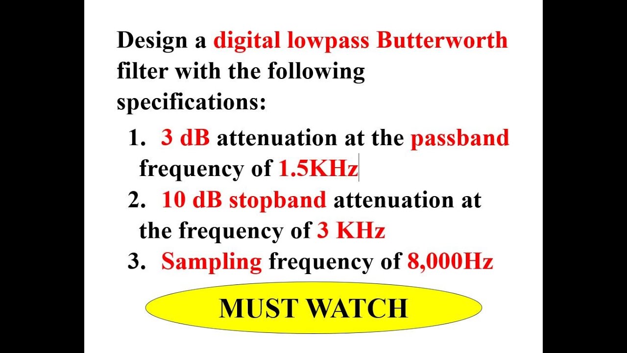
Q9a Design a digital lowpass Butterworth filter with the following specifications
7.4K
This comprehensive section covers the entire process of designing a digital Butterworth low-pass filter using given specifications. The workflow includes: (1) Converting digital frequencies from Hz to radians per second using ω = 2πF; (2) Calculating the sampling period T = 1/Fs; (3) Applying pre-warping technique to convert digital frequencies to analog domain using Ωa = (2/T) × tan(ωd × T/2); (4) Calculating low-pass prototype specifications Ωs_p = Ωa_s / Ωa_p; (5) Determining filter order using n = log10[(10^(A_s/10) - 1)/(10^(A_p/10) - 1)] / [2 × log10(Ωs_p)]; (6) Deriving the Butterworth prototype transfer function H_p(s); (7) Applying prototype transformation to obtain the analog filter transfer function; (8) Using bilinear transformation to convert the analog filter to its digital equivalent. For the given specifications (3 dB passband at 1.5 kHz, 10 dB stopband at 3 kHz, Fs = 8,000 Hz), the final digital transfer function is H(z) = [0.46 + 0.46z⁻¹]/[1 - 0.989z⁻¹].
Click to watch →
Butterworth Filter : Design of Low Pass and High Pass Filters
358.4K
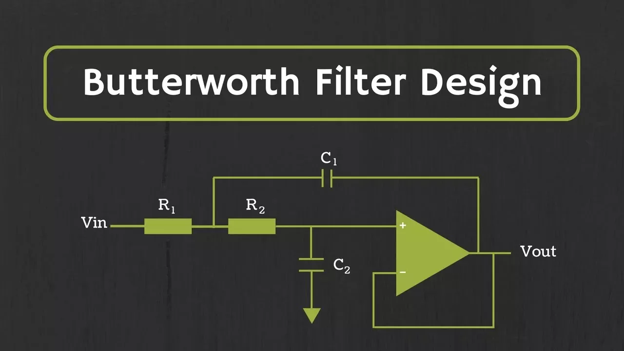
The Butterworth filter is characterized by its maximally flat frequency response in the passband, with a roll-off rate of 20n dB/decade for an nth-order filter. For a second-order Butterworth low pass filter, the quality factor Q must equal 0.707 to achieve this flat response, which can be implemented using the Sallen-Key filter topology with specific gain ratios (R4/R3 = 0.586). Higher-order Butterworth filters are designed by cascading multiple second-order sections, each satisfying the Q=0.707 condition, and the same polynomials used for low pass filters can be applied to high pass filters by simply interchanging capacitors and resistors in the circuit topology.
Click to watch →
Deep Dive
Implementing envelope detection algorithms, such as Root Mean Square (RMS) and moving average filters, to extract the smooth amplitude envelope of muscle activity.
![dr. R. Janča: Základy zpracování signálů (BAB31ZZS) – 11 [2. 12. 2024, ZS 24/25]](https://i.ytimg.com/vi/jprJuoPvxHg/maxresdefault.jpg)
dr. R. Janča: Základy zpracování signálů (BAB31ZZS) – 11 [2. 12. 2024, ZS 24/25]
439
Rectification (taking absolute value) followed by moving average filtering provides a simple method for envelope detection. The process: (1) take absolute value of the signal, (2) apply moving average filter to smooth the result. This creates a signal that tracks the amplitude envelope. The filter length determines the smoothing: longer windows provide more smoothing but less temporal resolution.
Click to watch →
![FREEEMG | Surface EMG fundamentals [Lesson 1]](https://i.ytimg.com/vi_webp/epvErjJoA3Q/maxresdefault.webp)
FREEEMG | Surface EMG fundamentals [Lesson 1]
3.5K
Envelope extraction removes non-reproducible components from raw EMG signals to reveal consistent activation patterns suitable for trial averaging and inter-subject comparison. Two primary algorithms serve this purpose: moving average (simple temporal averaging within user-defined windows) and root-mean-square (RMS, reflecting mean power and preferred per ISAAC guidelines). Time window selection critically impacts results—shorter windows (20ms) preserve rapid signal variations for dynamic movements, while longer windows (up to 500ms) smooth signals for static activities. Comparative analysis shows RMS preserves amplitude characteristics better than integration, making RMS the preferred choice. Time normalization converts absolute time scales to percentage-of-cycle representations, enabling comparison of muscle activation patterns across trials and subjects. For cyclical movements like gait analysis, time events must be defined to identify cycle boundaries (e.g., heel strike and toe-off). The process involves computing the envelope signal, identifying cycle events, normalizing each cycle to the mean cycle duration, and calculating mean and standard deviation across all cycles, transforming the time axis from seconds to 0-100%.
Click to watch →
SURFACE EMG SIGNAL ANALYSIS PART I BY DR SANJEEV GUPTA
3.1K
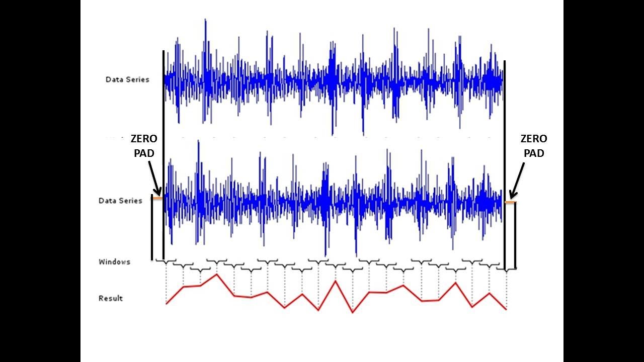
This video tutorial by Dr. Sanjeev Gupta demonstrates the complete workflow for analyzing surface electromyography (sEMG) signals using Delsys EMG Works software, covering signal acquisition, preprocessing (bandpass filtering), rectification to obtain absolute values, envelope estimation using moving RMS window, and event activation detection based on threshold methods for muscle activity analysis.
Click to watch →

ECE3311 Project 03 Overview (B-Term 2020)
121
AM envelope detection is implemented by squaring the AM signal, then applying a low pass filter, and finally taking the square root. Squaring the AM signal produces a signal with the message signal squared plus a DC component plus a double-frequency component. The low pass filter removes the double-frequency component, leaving the message signal squared plus DC. Taking the square root yields the original message signal.
Click to watch →

Surface Electromyography (SEMG) Signal Processing | Part 1
38.4K
To calculate the mean power (RMS envelope) of a SEMG signal, a moving average is taken of the filtered and rectified signal, followed by root mean square calculation over a specified window size. The window size affects the resulting signal characteristics: larger windows encompass more of the original signal but produce spikier, more distorted outputs; smaller windows result in flatter signals that do not reflect the peaks and variations of the original signal. Common window sizes range around 50 milliseconds, though there is no universally standard value.
Click to watch →
Deep Dive
Extracting key EMG features in both time and frequency domains (e.g., Mean Absolute Value, Zero Crossings, Median Frequency) to analyze muscle fatigue.
Kinesiological Electromyography – a practical guide to systems & assessment
3K
Four primary approaches analyze fatigue by transforming raw EMG signals into the frequency domain: (1) Mean frequency examines the central point of the frequency distribution, (2) Median frequency identifies the midpoint value (e.g., the 2000th sample in a 4000-sample set), (3) Zero crossing counts how many times the signal crosses the zero axis, decreasing as firing rates slow during fatigue, and (4) Mean amplitude looks for increases in signal magnitude as neuromuscular effort intensifies to maintain posture. Negative trends in the first three parameters indicate fatigue progression.
Click to watch →
Introduction to EMG Part 4
307
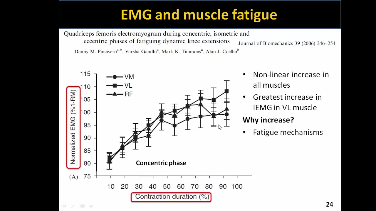
This section covers EMG frequency domain analysis for fatigue assessment. Converting time-domain EMG signals to frequency domain allows examination of median frequency changes. As fatigue ensues, median frequency decreases progressively and linearly, indicating a shift toward lower frequencies. The rate of decrease is greatest for rectus femoris, followed by vastus lateralis, then vastus medialis. This frequency drift is primarily caused by decreased conduction velocity of action potentials across muscle fiber membranes during fatigue. As muscle fibers fatigue, their ability to restore ion distribution decreases, prolonging action potential duration. Since frequency is inversely proportional to action potential length, this results in lower median frequencies, providing a measurable indicator of muscle fatigue.
Click to watch →

Prediction of muscle fatigue during dynamic exercises based on surface electromyography signals
189
Eight features were extracted: four from concentric phase and four from eccentric phase. These include: MAV (Mean Absolute Value), POW (Power), MDF (Median Frequency using Short-Time Fourier Transform), and WMDf (Median Frequency using Wavelet transforms). These features capture different aspects of muscle activation patterns during exercise.
Click to watch →

Eletromiografia - Conceitos Básicos
9.4K
Frequency domain analysis decomposes EMG signals into constituent frequencies, revealing motor unit characteristics. Median frequency analysis detects muscle fatigue: as fatigue develops, median frequency decreases because fatigued motor units fire at lower frequencies. This creates an abrupt frequency shift at metabolic thresholds correlating with respiratory compensation and lactate accumulation. The technique provides objective markers of fatigue progression, useful for exercise physiology and rehabilitation monitoring. Understanding these frequency shifts helps clinicians assess muscle endurance and fatigue resistance during functional activities.
Click to watch →

'EMG Signal Processing' by Dr Archana Kanawade
387
Frequency domain analysis reveals neuronal firing rates and muscle fatigue effects invisible in time domain. Mean and median frequencies shift toward lower frequencies during fatigue. Power spectral density analysis shows total power contributed by muscle activity, with increased power indicating greater contraction force. The power spectrum shifts toward higher frequencies during sustained contractions. Average instantaneous frequency analysis offers advantages over mean/median frequency methods but cannot handle sustained contractions. Key spectral features include maximum amplitude, mean amplitude, variance, RMS, number of peaks, and peak spectral density. EMG signals are inherently nonstationary, varying with person, time, and conditions. Time-frequency analysis provides localized spectral information. Short-Time Fourier Transform (STFT) provides spectral components within time windows but requires careful window size selection. Wavelet transform offers superior time-frequency resolution using scalable mother wavelets—providing good frequency resolution at low frequencies and better temporal resolution at high frequencies while maintaining constant area. Scale selection depends on dominant frequency or can use octave logarithmic steps. Single frequency CWT analysis can target specific frequencies of interest for efficient feature extraction.
Click to watch →
Deep Dive
Designing real-time myoelectric control applications, such as using processed EMG signals to control robotic grippers, prosthetics, or video games.

Myoelectric Prosthetic Design
384
Myoelectric prosthetic devices use electromyography (EMG) signals to detect muscle activity and control prosthetic movement; the process involves recording electrical signals from muscles using surface electrodes, applying signal processing techniques including filtration, rectification, and amplification to extract meaningful data, determining a threshold value to distinguish between muscle states (such as hand open versus closed), and using this processed signal to control servo motors that drive the prosthetic mechanism, demonstrating how mechatronic systems integrate biomechanical sensing with electronic control for functional prosthetic devices.
Click to watch →
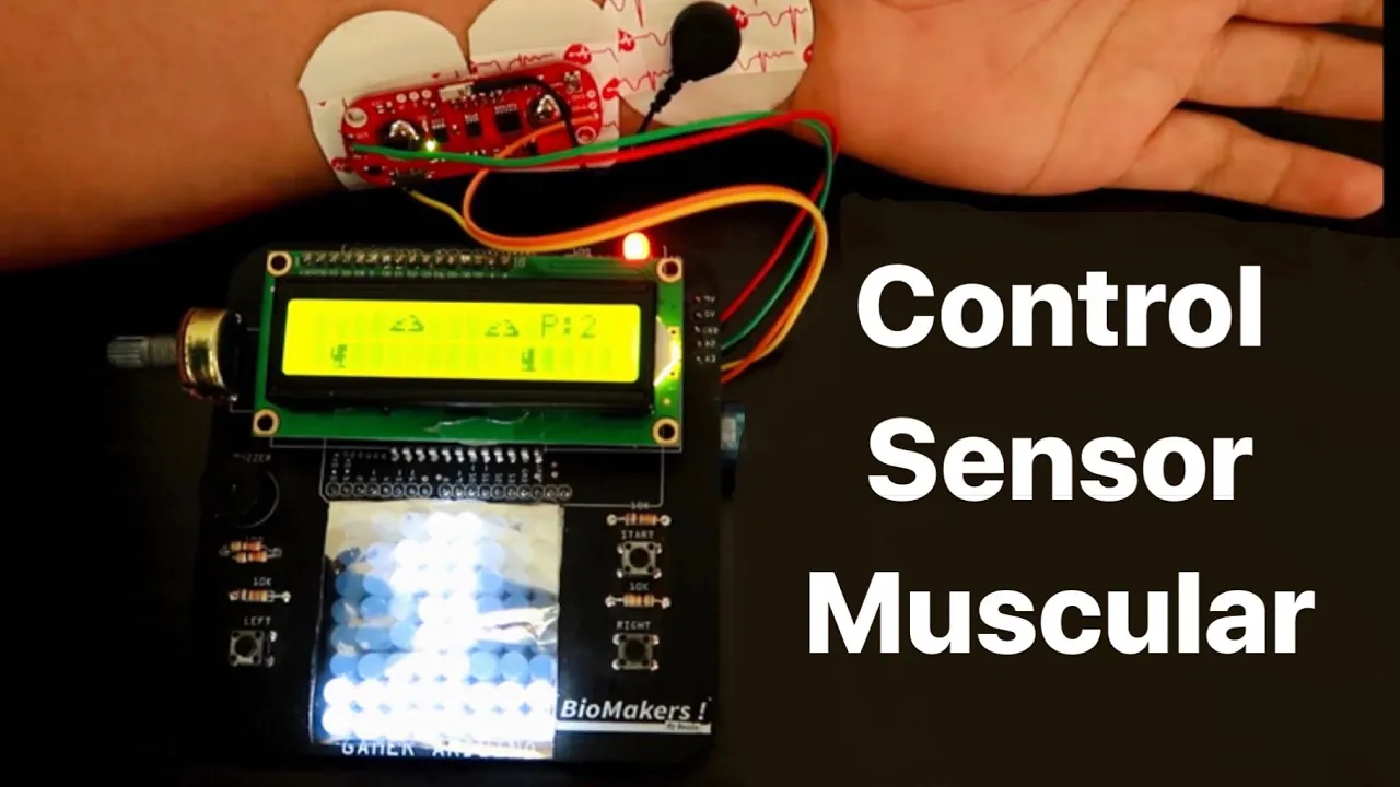
Arduino GOOGLE GAME Control EMG - PCBway
6.6K
This video demonstrates how to convert raw EMG (electromyography) muscle signals into digital game inputs by using a peak detection algorithm that identifies when muscle signals exceed a threshold value (50), replacing traditional button presses with muscle contractions to control game actions like jumping in a dinosaur game.
Click to watch →
![MANO ROBÓTICA [EMG] #1](https://i.ytimg.com/vi_webp/riCKxNn9AYE/maxresdefault.webp)
MANO ROBÓTICA [EMG] #1
3.6K
Electromyography (EMG) is a bioelectronic technology that captures and processes electrical signals generated by muscle contractions, enabling the development of myoelectric prosthetics (such as arms, hands, and legs) and human-machine interfaces for applications including video games, drones, and computer input devices; the technology works by using electrodes to detect electrical impulses from the musculoskeletal system, which are then amplified, filtered, and converted to digital signals for practical applications.
Click to watch →
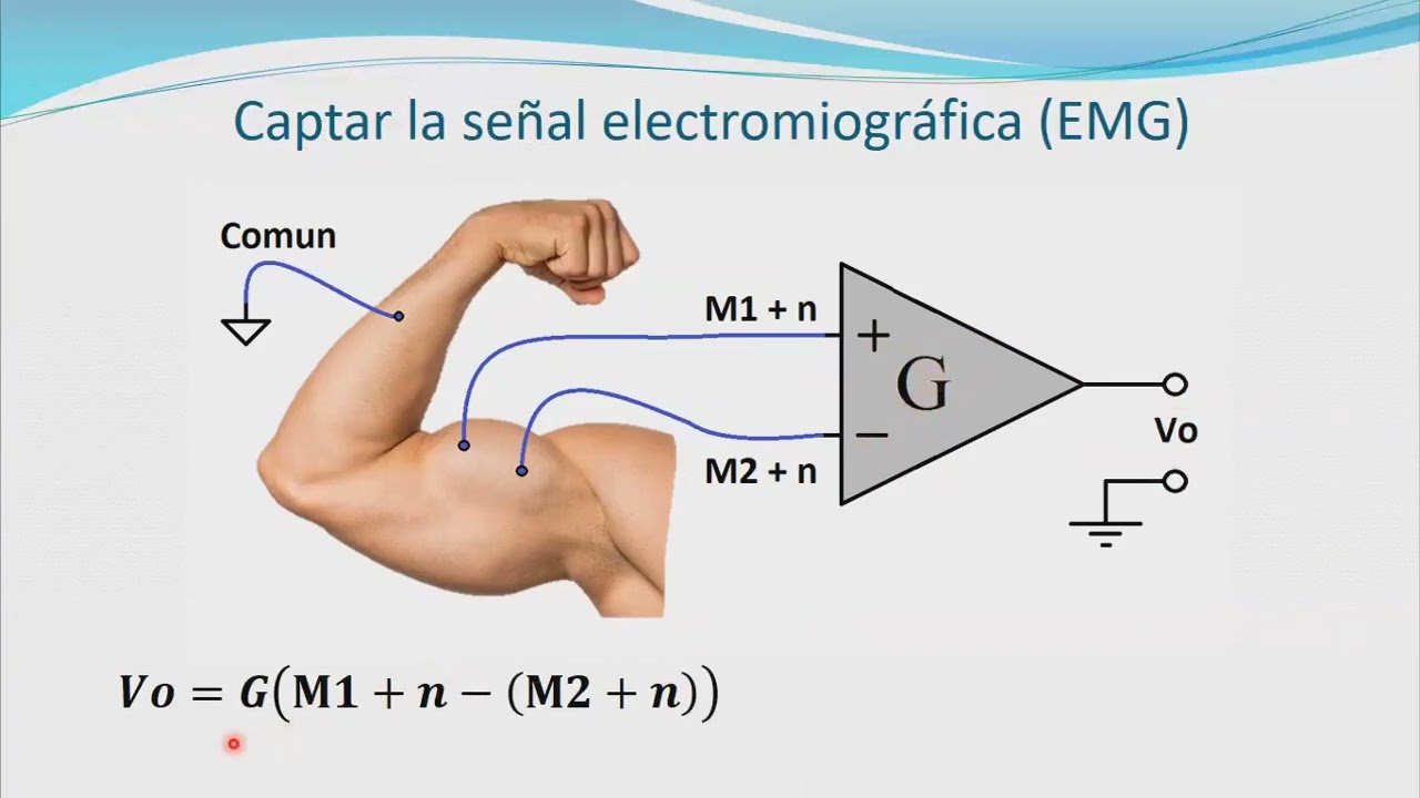
Introducción a la Biorrobótica - Control de Robots por interfaz neuronal
134
Raw EMG signals cannot be directly used for robotic control and require processing. The pipeline includes: (1) rectification to extract only the positive component of the signal, (2) amplification to increase signal strength, and (3) low-pass filtering to remove unwanted high-frequency components. A low-pass RC filter (220kΩ resistor and 1μF capacitor) extracts the muscle effort component. The cutoff frequency is calculated as 1/(2πRC), which is very low because the system is interested in the sum of impulses (muscle effort) rather than individual impulses. After rectification and filtering, the resulting signal represents integrated muscle effort, where amplitude directly corresponds to mechanical effort being generated by the muscle.
Click to watch →
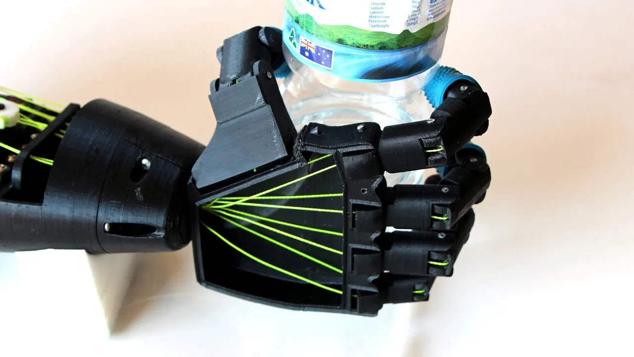
How I Designed & Built a Prosthetic Arm
195.9K
Electromyographic (EMG) sensors detect electrical signals generated when muscles contract. Surface electrodes placed on the skin pick up voltage changes across muscles during contraction. The harder a muscle is flexed, the higher the DC voltage output from the sensor circuit board. This signal can be processed to control prosthetic devices proportionally to the user's muscle effort.
Click to watch →
Start
Acceptance
External
Connection
Audience
Start
0:46- 1
Initiates the core discussion.
- 2
Sets the stage for main content.
Limitations of Time-Domain Rectification and the Necessity of Time-Frequency Analysis
While signal rectification is a classic, computationally simple method for estimating muscle activation amplitude, it has significant limitations. Rectification is a non-linear process that discards the phase information of the raw electromyography (EMG) signal and alters its spectral characteristics, potentially introducing artificial high-frequency artifacts. Critics argue that relying solely on rectified amplitude envelopes obscures critical physiological details. Alternative approaches, such as Wavelet Transforms, Hilbert-Huang Transforms, and autoregressive modeling, analyze the raw, unrectified signal. These advanced time-frequency methods are superior for detecting motor unit firing rates, identifying muscle fatigue, and decoding complex movement patterns for neural prosthetics—areas where simple rectified amplitude envelopes fail to provide sufficient diagnostic or control data.
Basic understanding of Electromyography (EMG) physiology, including how skeletal muscle contractions generate detectable biopotential signals.
Fundamentals of Arduino hardware operation, specifically analog-to-digital conversion (ADC) and configuring serial communication rates.
Core concepts of signal processing, such as raw signal amplitude, frequency, and the mathematical difference between alternating (AC) and direct (DC) components.
Basic proficiency in MATLAB programming, including data visualization, variable manipulation, and writing scripts to handle array operations.
Applying advanced digital filters, such as Butterworth bandpass and low-pass filters, to isolate the frequency bands of interest and reduce high-frequency noise.
Implementing envelope detection algorithms, such as Root Mean Square (RMS) and moving average filters, to extract the smooth amplitude envelope of muscle activity.
Extracting key EMG features in both time and frequency domains (e.g., Mean Absolute Value, Zero Crossings, Median Frequency) to analyze muscle fatigue.
Designing real-time myoelectric control applications, such as using processed EMG signals to control robotic grippers, prosthetics, or video games.
1.2K views8likes3:11@Challenger-TechOriginal Release: 2015-10-18
it's okay foreign so you
Up Next

22:35
Lithium Polymer Battery Safety: Safe Charging and Storage
@JoshuaBardwell
800.4K views•2022-06-21

12:54
Triumph of Orthodoxy Icon: Byzantine Art & History Explained
@BenCallan
2.1K views•2024-08-06

9:49
FastAPI vs Flask vs Django: Choosing the Right Python Web Framework
@TechWithTim
302.5K views•2024-05-26

1:42
Game of Thrones Opening Credits: A Cinematic Analysis
@gameofthrones
46.3M views•2011-04-18
Related Study Plans & Knowledge Roadmaps
Structured learning paths in General & Interdisciplinary Studies
general-studies
Elevator Engineering: History, Physics & Cities
01From Hoists to Safety Brakes: The Dawn of Vertical Lift
02Hydraulic vs. Traction: The Engineering Physics of Elevators
03Modern Speed, Safety, and Algorithms
+ 2 more learning modules
12h5 modules
Explore Roadmap
general-studies
Rubber: Material Science, History & Geopolitics
01Origins of Natural Rubber & Mesoamerican History
02The Chemistry of Natural Rubber & Vulcanization
03The Geopolitics of the Rubber Boom & Colonization
+ 2 more learning modules
12h5 modules
Explore Roadmap
general-studies
Containerization: Evolution, Logistics & Trade
01Ancient Trade & Bulk Cargo: Amphorae to Barrels
02The Industrial Revolution & Cardboard Packaging
03The Containerization Revolution: Malcom McLean
+ 2 more learning modules
12h5 modules
Explore Roadmap
general-studies
Textile Tech: Evolution, Labor & Global Impact
01Pre-Industrial Textiles: Handloom & Cottage Industry
02Mechanization: The Spinning Jenny to the Power Loom
03The Factory System & Global Labor Transformation
+ 2 more learning modules
10h5 modules
Explore Roadmap