Hand-eye calibration is a technique that establishes the mathematical transformation between a camera mounted on a robot's end-effector and the robot's coordinate frame, enabling the robot to translate 2D pixel coordinates from camera images into precise 3D positions in the world frame, which is essential for achieving sub-millimeter precision in applications like automated assembly.
Robotic Hand-Eye Calibration: Precision Alignment Demo
Added:Deep Dive
Fundamentals of coordinate transformations, including homogeneous transformation matrices, 3D rotations, and translation vectors.
An Introduction to Homogeneous Transformations (Theory and Formulation)
440
A coordinate system consists of an origin and three orthogonal basis vectors (X, Y, Z) following the right-hand convention. Euclidean transformations combine translation (adding values to coordinates) and rotation (using trigonometric functions). Homogeneous transformation matrices combine rotation and translation into a single 4x4 matrix: the top-left 3x3 submatrix represents rotation, the rightmost column represents translation, and the bottom row is always [0, 0, 0, 1]. Rotation matrices about X, Y, and Z axes have specific structures where the rotation axis column remains unchanged with a 1, and the perpendicular axes are transformed using cosine and sine terms. The sine term in the row perpendicular to the rotation axis is always negative.
Click to watch →

Module Rob chapitre 2 partie 1/4
14K
Homogeneous coordinates extend 3D Cartesian coordinates to 4D by adding a fourth coordinate (1 for points, 0 for directions). A homogeneous transformation matrix is a 4x4 matrix containing a 3x3 rotation submatrix and a 3x1 translation vector. The rotation submatrix contains the unit vectors of the target frame expressed in the source frame, while the translation vector contains the position of the target frame's origin. This unified representation allows coordinate transformations through matrix multiplication and enables the matrix to be invertible while preserving geometric properties.
Click to watch →

Homogeneous Transformation 7
5.7K
Homogeneous transformation matrices are 4x4 matrices used to represent rigid body transformations in 3D space. They consist of a 3x3 rotation matrix in the upper-left corner and a 3x1 translation vector in the rightmost column, with the bottom row always being [0 0 0 1]. There are two main types: pure translation (only movement, no rotation) and pure rotation (only rotation, no movement). In pure translation, the rotation matrix becomes the identity matrix, and only the translation vector changes. In pure rotation, the translation vector remains zero, and only the rotation matrix changes. The matrix multiplication process involves multiplying the rotation matrices and adding the translation vectors to calculate new positions.
Click to watch →

Homogenous Transformation Matrix 3D مصفوفة التحويل المتجانسة
1.2K
This comprehensive section covers the foundational concepts of 3D coordinate systems and transformations. The right-hand rule establishes axis orientation: thumb along X-axis, index finger along Y-axis, middle finger along Z-axis. This rule determines positive/negative rotation directions. X-axis rotations keep X fixed while Y and Z move; Z-axis rotations keep Z fixed while X and Y move. Translation moves along axes using 4x4 matrices with values in the last column. The rotation matrices differ by axis: X-axis [[1, 0, 0], [0, cosθ, -sinθ], [0, sinθ, cosθ]], Y-axis [[cosθ, 0, sinθ], [0, 1, 0], [-sinθ, 0, cosθ]], Z-axis [[cosθ, -sinθ, 0], [sinθ, cosθ, 0], [0, 0, 1]].
Click to watch →

SLAM-Course - 02 - Homogeneous Coordinates (2013/14; Cyrill Stachniss)
80.8K
Transformations in homogeneous coordinates are expressed as matrix multiplications: x' = Mx, where M is the transformation matrix. Translation uses a 4x4 matrix with the form: [[1, 0, 0, 0], [0, 1, 0, 0], [0, 0, 1, 0], [Tx, Ty, Tz, 1]], where the top-left 3x3 block is an identity matrix and the fourth column contains the translation vector. Rotation matrices in homogeneous coordinates use the same matrices as in Cartesian coordinates. For 2D rotation around the origin by angle θ: [[cos(θ), -sin(θ), 0], [sin(θ), cos(θ), 0], [0, 0, 1]]. For 3D rotations, there are three standard rotation matrices around the x, y, and z axes. A rigid body transformation combines rotation and translation into a single 4x4 matrix: [[R, T], [0, 1]], where R is a 3x3 rotation matrix and T is a 3x1 translation vector. This matrix has 6 parameters (3 for rotation, 3 for translation) and represents the complete motion of an object in 3D space.
Click to watch →
Deep Dive
Basic computer vision principles, particularly camera calibration, intrinsic and extrinsic parameters, and the pinhole camera model.
Computer Vision, F23: Camera Model, Calibration, Depth Inference, Panorama Image, Fundamental Matrix
410
The pinhole camera model represents a camera as a single point (optical center) in 3D space. Light rays pass through this point to form an image on the image plane. The distance between the lens and image plane is the focal length F. Using the intercept theorem, 3D coordinates (x, y, z) map to 2D image coordinates (u, v) through u/x = F/z and v/y = F/z. Homogeneous coordinates add a scale factor to Cartesian coordinates, enabling matrix representation of projective transformations. When the camera is not at the origin and its axes are not aligned with the 3D space, rotation and translation are needed. The complete camera projection combines intrinsic and extrinsic parameters: [K, 0; 0, 1] * [R, t; 0^T, 1] = [KR, KT; 0, 1]. Camera calibration finds the parameters of the mapping matrix M = [KR, KT; 0, 1]. Intrinsic parameters (f/s, ou, ov) describe the camera's internal characteristics, while extrinsic parameters (R, t) describe the camera's position and orientation in the 3D world. The calibration equations form a linear system that can be solved using Cramer's rule. Once M is known, it can be decomposed to find individual parameters using the orthogonality properties of rotation matrices.
Click to watch →

CVFX Lecture 17: Image formation and single-camera calibration
70.9K
The pinhole camera model describes basic image formation: light passes through a small aperture and projects an inverted image onto a sensor plane. In computer vision, we assume the image plane sits in front of the camera center for convenience. The distance between the camera center and image plane is the focal length (f). Using similar triangles, the pinhole projection equations relate 3D world coordinates (X,Y,Z) to 2D image coordinates: x = f*X/Z and y = f*Y/Z. The camera calibration matrix K = [[α_x, 0, x₀], [0, α_y, y₀], [0, 0, 1]] encapsulates internal parameters: α_x = f/dx and α_y = f/dy represent focal lengths in pixel units, while (x₀, y₀) is the principal point. Real cameras exhibit radial lens distortion where points bulge outward from the center, modeled as x_distorted = x(1 + k₁r² + k₂r⁴).
Click to watch →

Lec-34_Intrisic and Extrinsic parameters , Lens Distortion | Computer Vision | IT/ICT Engineering
1.8K
Camera calibration involves determining both intrinsic parameters (focal length, principal point, scale factors, and skew angle) that define the projective transformation from 3D camera coordinates to 2D image coordinates, and extrinsic parameters (rotation matrix R and translation vector t) that represent the rigid transformation from the 3D world coordinate system to the camera coordinate system; additionally, radial lens distortion is modeled using polynomial coefficients k₁, k₂, and k₃ to correct image warping effects, while direct parameter calibration provides a unified approach for simultaneously recovering all camera parameters.
Click to watch →
#59 Camera Intrinsics & Extrinsics | Part 1 | Modern Computer Vision
1.5K
Camera calibration involves determining two fundamental parameter sets: intrinsics (internal camera properties like focal length and optical center) and extrinsics (camera position and orientation relative to the world). The pinhole camera model describes how 3D points project onto 2D image planes using perspective projection equations, where image coordinates depend on the ratio of scene coordinates to depth (x = f × xc/zc, y = f × yc/zc). A special case called rotational homography allows stitching images of 3D scenes when only pure rotation occurs without translation, as this eliminates parallax effects that would otherwise prevent a single homography from working across different viewpoints.
Click to watch →
Lecture 6: Camera Model (KAIST CS479, Spring 2025)
807
The complete camera model combines intrinsic and extrinsic parameters. The intrinsic 3×3 matrix encodes focal length and principal point for projecting camera coordinates to image coordinates. The extrinsic 3×4 matrix (rotation + translation) transforms world coordinates to camera coordinates. Together they form the full camera matrix P. Camera calibration determines these parameters from 3D-to-2D correspondences by solving homogeneous linear systems derived from the cross-product constraint that P·X and x must be parallel vectors.
Click to watch →
Deep Dive
Robot kinematics, specifically forward kinematics, to understand how a robot tracks its own end-effector pose.
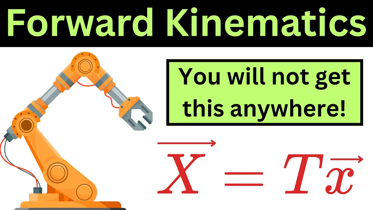
Solved Example - Forward Kinematics
38.1K
Forward kinematics is the process of determining where the tip of a robot's arm (called an endeffector, such as a gripper) ends up in a fixed coordinate frame when you translate and rotate each of its joints. It involves calculating the position and orientation of the endeffector based on the joint angles and link lengths.
Click to watch →

Robotica #7: CINEMATICA, le convenzioni di Denavit-Hartenberg
1.5K
The complete forward kinematics matrix T includes transformations from the base frame to the end-effector frame. The base frame may not coincide with the DH frame 0, requiring an additional transformation matrix. The end-effector frame transformation (T_n) from the last DH frame to the actual end-effector frame is a constant matrix describing the tool position relative to the robot's last joint. The end-effector pose is represented by a 4x4 matrix containing a 3x3 rotation matrix (orientation of end-effector axes n, s, a) and a 3x1 translation vector (position of end-effector origin).
Click to watch →

EME454-Lec9 -part1
124
Forward kinematics is the mathematical method that transforms joint angles (joint space) into the position and orientation of a robot's end effector in Cartesian space, enabling robots to understand their own position and perform precise tasks like simulation, trajectory planning, control systems, and workspace analysis.
Click to watch →
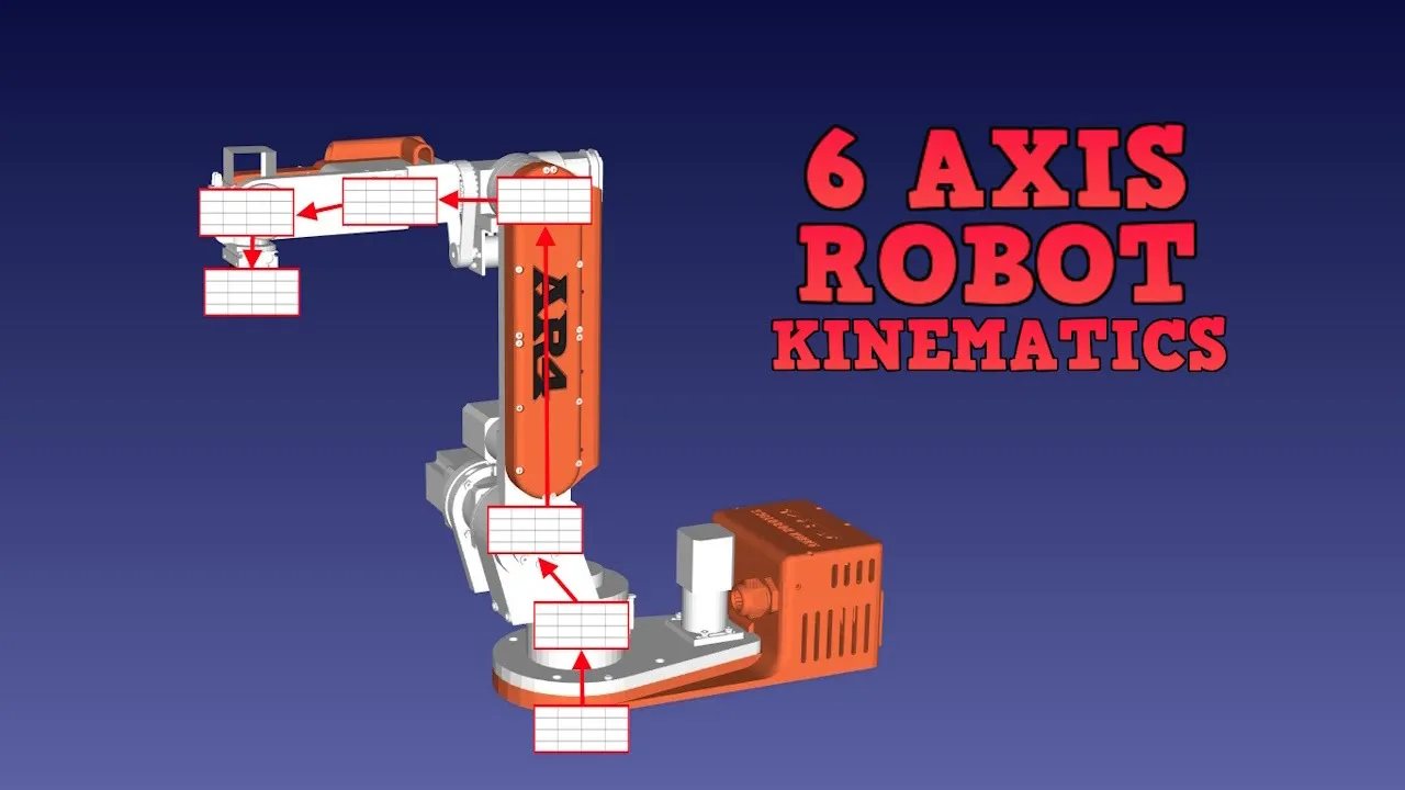
6 Axis Robot Forward & Inverse Kinematics Tutorial - Denavit Hartenberg Parameters With the AR4-MK2
59.9K
Robot kinematics involves calculating the relationship between joint angles and end-effector position/orientation; forward kinematics determines Cartesian coordinates from joint angles using homogeneous transformation matrices derived from Denavit-Hartenberg parameters (theta, alpha, d, a), while inverse kinematics solves for joint angles from desired Cartesian positions by first finding the spherical wrist center position geometrically and then solving for wrist orientation, with singularities requiring configuration values to resolve ambiguous solutions.
Click to watch →
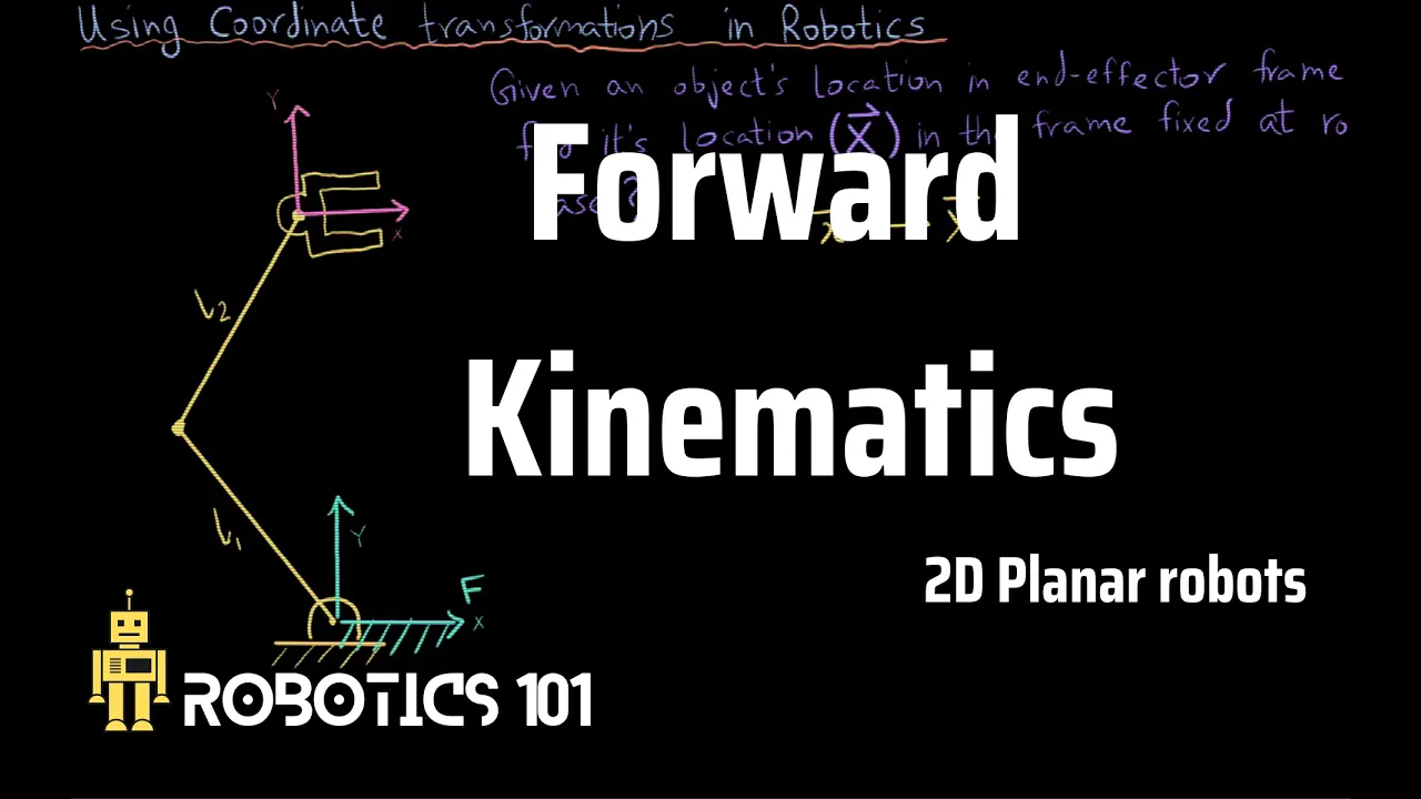
Forward Kinematics of robots | Planar 2D robots | Robotics 101
34.2K
Forward kinematics determines the position and orientation of a robot's end-effector in space by applying coordinate transformations through a series of rotation matrices and displacement vectors, calculated from given link lengths and joint angles using the relationship X_big = A₁A₂A₃X_small, where the rotation matrix contains the sum of joint angles for orientation and the displacement terms provide the Cartesian coordinates of the end-effector.
Click to watch →
Deep Dive
Basic linear algebra and optimization techniques, such as solving systems of equations and least-squares fitting.
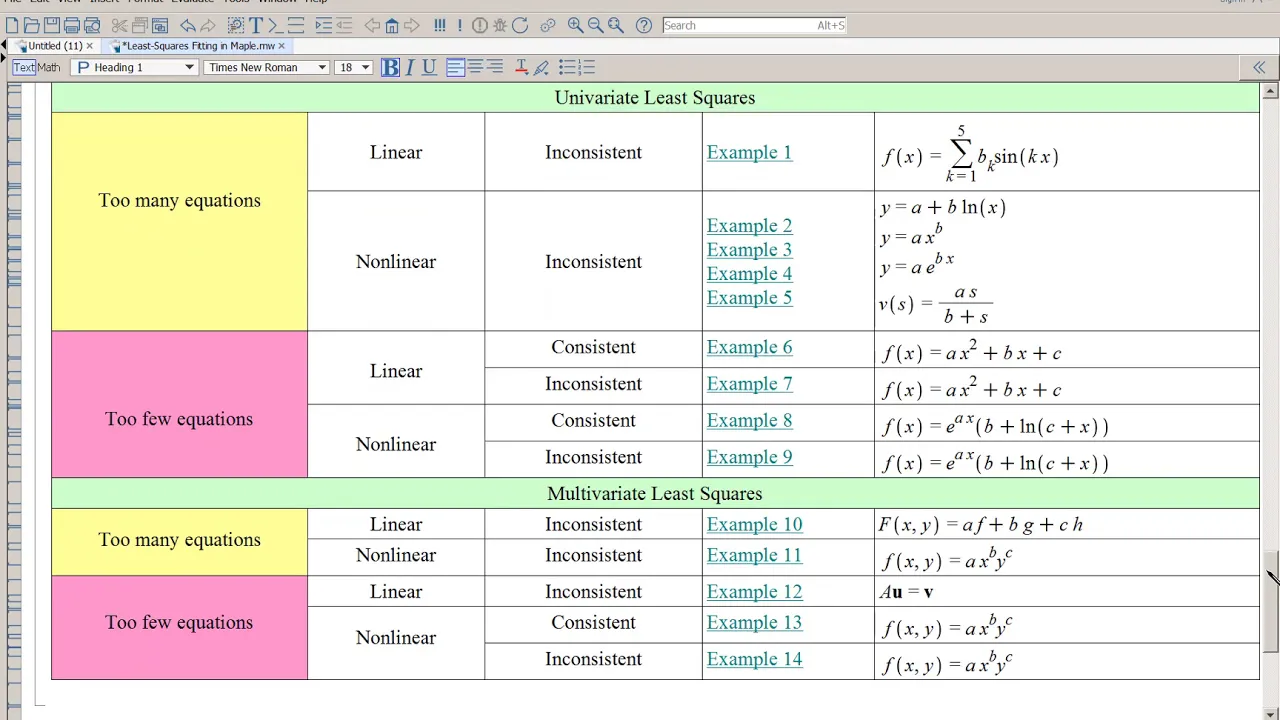
Least-Squares Fitting in Maple
4.3K
The Linear Algebra package converts problems to matrix-vector form Ax=B using GenerateMatrix. The least squares command returns parameter values directly. The Optimization package's LS solve command accepts residual lists and returns sum of squares and parameters. Different packages return different formats: equations, vectors, or optimization results.
Click to watch →
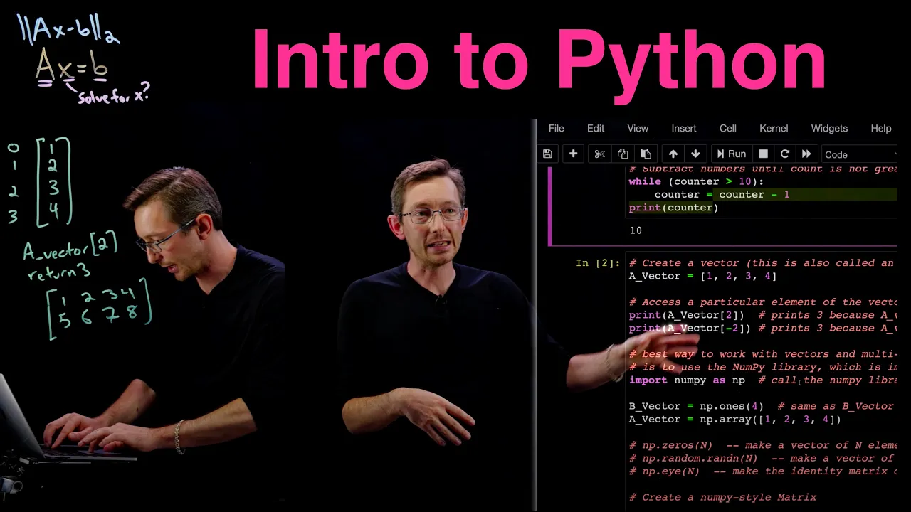
Engineering Math Pre-Req: Quick and Dirty Introduction to Python
99.6K
Numpy's linear algebra module (np.linalg) provides least squares solutions for solving systems of equations Ax = B. The function np.linalg.lstsq() finds the x that minimizes ||Ax - B||₂, the Euclidean norm of the residual. This method works even when the system is overdetermined (more equations than unknowns) or underdetermined, finding the best approximate solution. The solution can be verified by computing A @ x - B, which should yield values close to zero.
Click to watch →

Line Fitting With Least Squares- Linear Algebra
462
Line fitting is a numerical method that uses linear algebra to find the best-fitting line (y = mx + b) for a given dataset by constructing an overdetermined linear system (A matrix with ones and X values, B vector with Y values) and solving it using the method of least squares to minimize the error between the model predictions and observed data.
Click to watch →
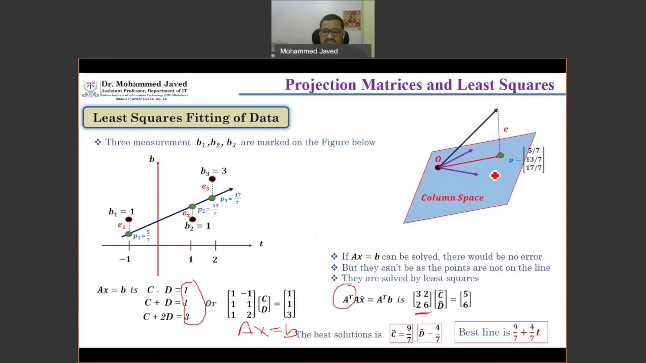
Least Square Fitting or Regression Line Fitting using ALGEBRA and CALCULUS, Quadratic Curve fitting
274
Least square fitting is a mathematical technique used to find the best-fit line or curve through a set of data points by minimizing the sum of squared errors between the observed values and the predicted values; this can be solved algebraically using the normal equations (A^T A)x = A^T b, which transforms the rectangular system into a solvable square system, or through calculus by taking partial derivatives of the error function with respect to the unknown coefficients and setting them to zero, with the same optimal solution being obtained regardless of the method chosen.
Click to watch →

Least square fit and Eigen Values and Vectors
195
The least squares linear fit finds the best-fitting line for data by minimizing squared errors. The process involves: (1) writing data in matrix form Ax = B, (2) multiplying both sides by A^T to get A^T A x = A^T B (normal equations), (3) computing A^T A and A^T B, (4) finding the inverse of A^T A, and (5) solving for x by multiplying (A^T A)^(-1) by A^T B. This method provides the optimal parameters M and C for the line y = Mt + C.
Click to watch →
Prerequisite Knowledge
- Concept 01Fundamentals of coordinate transformations, including homogeneous transformation matrices, 3D rotations, and translation vectors.
- Concept 02Basic computer vision principles, particularly camera calibration, intrinsic and extrinsic parameters, and the pinhole camera model.
- Concept 03Robot kinematics, specifically forward kinematics, to understand how a robot tracks its own end-effector pose.
- Concept 04Basic linear algebra and optimization techniques, such as solving systems of equations and least-squares fitting.
Subsequent Learning
- Step 01Deep dive into the mathematical formulations of hand-eye calibration (solving the AX = XB or AX = YB matrix equations).
- Step 02Visual Servoing (both Position-Based and Image-Based), which uses real-time vision feedback to dynamically guide robotic motion.
- Step 033D object pose estimation and perception algorithms using depth sensors or point clouds (e.g., Iterative Closest Point algorithm).
- Step 04Application of calibrated vision systems in industrial tasks requiring sub-millimeter precision, such as PCB soldering, bin-picking, and robotic surgery.
Calibration Basics
Precision Demo
Calibration Basics
0:02Playing Section
- 1
Explains camera distortion types and their impact on measurement accuracy.
- 2
Defines intrinsic parameters needed to correct image geometry.
- 3
Introduces hand-eye calibration for relating camera vision to robot movement.
Calibration-Free End-to-End Learning and Visual Servoing
While traditional hand-eye calibration relies on precise, rigid mathematical models and offline calibration targets, it is highly sensitive to physical disruptions and environmental changes, requiring frequent recalibration. A major alternative perspective advocates for calibration-free approaches, such as end-to-end deep reinforcement learning and uncalibrated visual servoing. Instead of explicitly calculating the geometric transform between the camera and the robot, these methods train the system to map raw visual inputs directly to motor commands. This closed-loop feedback mechanism mimics biological systems, offering greater adaptability, robustness to camera shifts, and the ability to operate in dynamic, unstructured environments where sub-millimeter geometric calibration is impractical to maintain.
Deep Dive
Deep dive into the mathematical formulations of hand-eye calibration (solving the AX = XB or AX = YB matrix equations).
Matthew Giamou on Convex Relaxations for Geometric Problems in Robotics | Toronto AIR Seminar
943
Hand-eye calibration determines the extrinsic transformation between a robotic hand and camera using the AX=XB formulation. This applies to any sensor measuring ego motion, including monocular cameras lacking scale information. The problem requires determining SE(3) transformations from SO(3) rotation matrices defined by quadratic orthogonality constraints. Certification of solutions provides complementary safety guarantees beyond probabilistic uncertainty measures, essential for multi-sensor robotic systems.
Click to watch →

Lecture 9 Visual Servoing
5.3K
Hand-eye calibration determines the relative transformation between the camera and robot end effector, essential for converting camera-based control commands to robot joint velocities. The mathematical formulation solves AX = XB for multiple observations, where A represents relative robot poses and B represents relative camera poses relative to a calibration pattern. Practical implementation involves moving the robot to multiple positions, recording end effector poses and corresponding camera poses relative to the pattern, then solving for the constant transformation X that satisfies all observations. This calibration enables accurate visual servoing by establishing the coordinate relationship needed for effective control.
Click to watch →

3 - MoveIt - Easy Hand Eye Calibration with MoveIt
24.5K
Hand-eye calibration determines the spatial relationship between a robot arm and a mounted camera using the AX=XB equation, where A represents camera motion between poses, B represents robot motion, and X is the unknown transform to solve; MoveIt Calibration provides an easy-to-use GUI that automates this process by collecting transform data from multiple robot poses and applying AX=XB solvers to recover the camera-to-end-effector transform for both eye-in-hand and eye-to-hand configurations.
Click to watch →
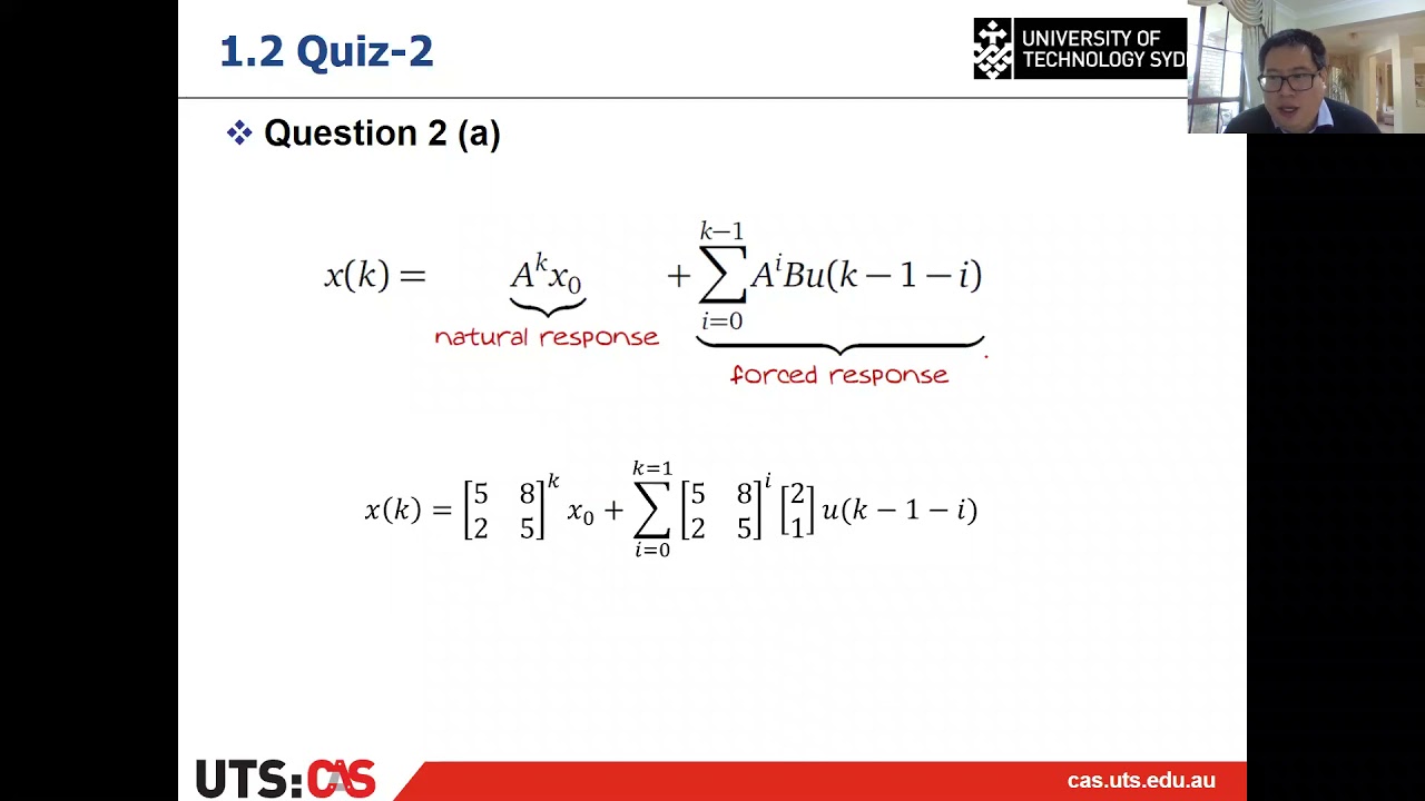
Lecture 10 Subject Review
320
Visual servoing minimizes error between desired and current feature locations. The control law derives as: calculate error e = s* - s, set error derivative ẋ = -λe, solve for camera velocity vc = -λLE⁺e where LE is the feature Jacobian mapping 6D camera velocity to 2D feature velocity. Hand-eye calibration solves AX = XB to determine camera-end-effector pose, where A is camera-end-effector pose (from checkerboard) and B is end-effector-base pose (from kinematics), enabling conversion of camera velocity commands to end-effector velocity commands.
Click to watch →
RI Seminar: Gregory S. Chirikjian : Stochastic Models in Robotics
4.3K
Ultrasound probe calibration requires determining the transformation between the image plane (which can float relative to the physical probe) and a reference frame attached to the probe. This is formulated as the AX=XB problem where A represents transformations from the global tracker to the probe, B represents transformations from the global tracker to the image plane, and X is the unknown transformation relating the probe reference frame to the image plane. The solution requires matching relative motions derived from phantom patterns.
Click to watch →
Deep Dive
Visual Servoing (both Position-Based and Image-Based), which uses real-time vision feedback to dynamically guide robotic motion.
25: Canny-Kantendetektor, Visual Servoing, Punktwolken
1.2K
Visual servoing uses visual feedback to control robot motion, compensating for kinematic errors, sensor inaccuracies, and execution errors. Two main configurations exist: external cameras (fixed in environment) and onboard cameras (mounted on robot arm). Position-based visual servoing determines 3D object positions from visual features and transforms them to robot coordinates, generating motion commands to reach target positions. Image-based visual servoing controls motion based on differences between current and desired image configurations, abstracting away explicit 3D reconstruction. The image Jacobian matrix relates 3D point velocities to image plane velocities, enabling control law derivation as v = J⁺(x)ᵀe. Modern systems combine visual, force, and joint encoder data for robust manipulation in unstructured environments.
Click to watch →

Emisión en directo de Programa Institucional de Divulgacion
105
Two main visual servoing approaches exist: image-based and position-based. Image-based control uses features directly in image space, calculating errors between desired and actual positions to generate velocity commands. This approach is robust to calibration errors but produces non-intuitive movements. Position-based control converts features to 3D coordinates before generating commands, requiring accurate calibration but producing more intuitive movements. The interaction matrix maps camera motion to feature motion in image space, enabling appropriate control command generation.
Click to watch →

Image-Based Visual Servoing - Robot Control Part 1
8K
Two main approaches exist for visual servoing: Position-Based Visual Servoing (PBVS) reconstructs 3D object geometry from multiple images taken at different viewpoints, then controls the robot based on this 3D model; Image-Based Visual Servoing (IBVS) controls the robot directly using 2D image features without explicit 3D reconstruction. PBVS uses structure from motion techniques to triangulate 3D feature points and create surface models, while IBVS focuses on specific feature points and defines desired positions for them. Blob detection calculates centroid location and orientation using moments of inertia. Feature point matching algorithms like SIFT and SURF detect distinctive points robust to rotation, scaling, and translation, enabling correspondence between images. IBVS avoids the computational complexity of 3D reconstruction while still achieving precise visual guidance.
Click to watch →

IBVS and PBVS Used in a 2DOF Robot
595
This video demonstrates two visual servoing approaches for controlling a 2-degree-of-freedom planar robot arm to center a specific world point in the camera image. In Image-Based Visual Servoing (IBVS), the system directly uses pixel coordinate errors to compute end-effector velocity commands through the interaction matrix L, requiring direct velocity control. In Position-Based Visual Servoing (PBVS), the desired image coordinates are back-projected into world coordinates to determine the desired camera pose, then joint angles are computed using inverse kinematics and controlled via feedback linearization with PD control. IBVS offers faster computation and better tolerance to model errors, while PBVS provides higher accuracy in world coordinates and works with torque-controlled robots lacking direct velocity control.
Click to watch →

Colloque Technologique Susan Calvin - Boris Morinière - AIRBUS
147
Traditional fuselage assembly uses laser trackers requiring 2+ hours per setup. Airbus developed visual servoing with multiple cameras for real-time point tracking at 10Hz, enabling dynamic positioning to achieve 0.1-0.5mm tolerances. The system calculates errors directly in the image plane without camera calibration, simplifying setup. Combined with profilometers for flush verification and global measurements for warping detection, setup time reduced from hours to under 2 minutes. This represents a fundamental shift from point-by-point scanning to continuous visual feedback control.
Click to watch →
Deep Dive
3D object pose estimation and perception algorithms using depth sensors or point clouds (e.g., Iterative Closest Point algorithm).

From Point Clouds to 3D Poses: How to Perform ICP with Open3D in Python
15.8K
The Iterative Closest Point (ICP) algorithm is a local registration technique used to estimate the pose (position and orientation) of an object point cloud relative to a scene point cloud by iteratively finding nearest-point correspondences and computing transformations; unlike global registration, ICP requires a reasonable initial guess of the object's position, and its performance can be significantly improved by using point-to-plane ICP (which utilizes surface normals) rather than point-to-point ICP, achieving better alignment with fewer iterations.
Click to watch →
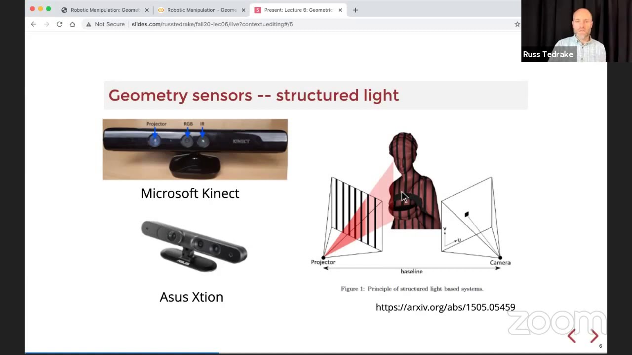
Lecture 6 | MIT 6.881 (Robotic Manipulation), Fall 2020 | Geometric Perception (Part 1)
3.2K
Geometric perception enables robots to estimate object poses by matching 3D point clouds from depth sensors (like Intel RealSense cameras) to known object models, using mathematical optimization techniques such as Singular Value Decomposition (SVD) to solve the inverse kinematics problem of finding the best rigid transformation that aligns observed scene points with model points, with the Iterative Closest Point (ICP) algorithm providing an iterative refinement approach that alternates between assigning correspondences and optimizing the pose estimate.
Click to watch →

Lecture 6: MIT 6.800/6.843 Robotics Manipulation (Fall 2021) | "Geometric Perception (Part 2)"
1.5K
This lecture continues geometric perception, connecting to kinematics work on robot motion. The major theme is estimation with messy point clouds. RGBD sensors (like D415) provide color and depth images transformed into point clouds. The Iterative Closest Point (ICP) algorithm alternates between optimizing pose given correspondences and finding correspondences given pose. Each subproblem has a global optimum, but alternation can cause local minima. This is a common pattern in optimization, seen in EM algorithm and bilinear optimization.
Click to watch →

Iterative Closest Point (ICP) - Computerphile
151.6K
The Iterative Closest Point (ICP) algorithm is a popular method for aligning point clouds by iteratively finding correspondences between points in two sets and optimizing the translation and rotation to minimize distances between matched points, though it may converge to local minima if initial estimates are poor.
Click to watch →
Point Cloud Alignment using ICP (See 2021 Video die to audio issues in this video)
28.3K
The Iterative Closest Point (ICP) algorithm is a fundamental technique for aligning 3D point clouds by iteratively finding correspondences between points and computing the optimal transformation (rotation and translation) to minimize the squared error between corresponding points; the algorithm works by first computing the center of mass of both point clouds, then using Singular Value Decomposition (SVD) to solve the orthogonal Procrustes problem for the rotation matrix, and finally applying the transformation to align the point clouds, with the process repeating until convergence or until the error falls below a threshold.
Click to watch →
Deep Dive
Application of calibrated vision systems in industrial tasks requiring sub-millimeter precision, such as PCB soldering, bin-picking, and robotic surgery.

Bin Picking y control de soldadura Bcnvision
235
This video demonstrates how artificial vision systems enable automated metal processing through two key applications: 3D bin picking uses 3D scanning and matching to locate and coordinate robotic arms for picking metal pieces, while 3D profile measurement combined with Deep Learning enables comprehensive weld inspection by capturing complete weld images and detecting defects, and pericentric optics with Deep Learning allows inspection of internal thread features without physical access.
Click to watch →
![Introducing Industrial AI and 3D Vision Solutions | Webinar [November 2020]](https://i.ytimg.com/vi/cnnxS5duos0/hqdefault.jpg)
Introducing Industrial AI and 3D Vision Solutions | Webinar [November 2020]
4.8K
Calibration is a critical challenge in bin picking applications. Modern vision systems provide automated calibration interfaces that simplify the process: users simply take approximately 15 pictures of the workspace, and the system calculates and validates robot and scanner parameters. After capturing reference points, the interface indicates whether calibration was successful or if adjustments are needed, significantly reducing setup time and complexity.
Click to watch →
PnP Calibration with Computer Vision!
46.7K
Vision calibration in pick and place machines improves placement accuracy by using computer vision to detect and correct for component position and rotation errors that occur during the picking process, compensating for tolerance stack-up from feeders, nozzles, and mechanical systems; this is achieved through three main calibration types: lens distortion correction (flattening image warping), fiducial calibration (aligning the board coordinate system), and bottom vision (detecting component position and rotation on the nozzle).
Click to watch →
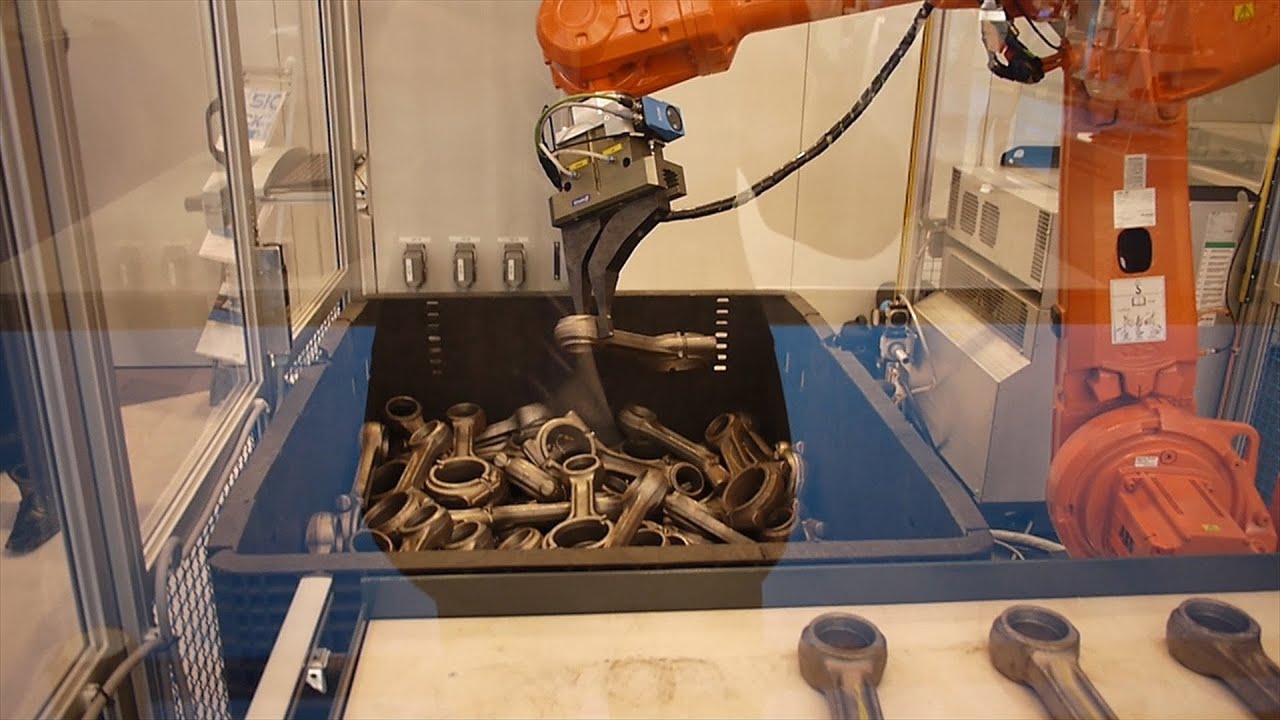
PLB vision system from SICK: Part localization in bins for robotic bin-picking | SICK AG
40.4K
A 3D vision system for robotic bin-picking uses CAD-based 3D shape matching to precisely locate randomly oriented parts in bins, enabling robots to identify and pick parts efficiently by calculating optimal gripping positions based on part geometry and verifying clear access points before execution.
Click to watch →

How to Set Up FANUC iRVision 2D Guided Place to Accurately Place Objects
18.1K
Vision system calibration establishes the mapping between pixel coordinates (vision system output) and millimeter measurements (robotics coordinate system). Since vision systems operate in pixels while robots work in millimeters, calibration creates a transformation matrix that converts between these coordinate systems. The calibration process requires providing corresponding pixel and millimeter data points, after which the vision software computes the transformation. This mapping enables accurate position reporting from vision detection to robot motion commands, forming the foundation for all guided placement applications.
Click to watch →
Calibration Basics
Precision Demo
Calibration Basics
0:02- 1
Explains camera distortion types and their impact on measurement accuracy.
- 2
Defines intrinsic parameters needed to correct image geometry.
- 3
Introduces hand-eye calibration for relating camera vision to robot movement.
Calibration-Free End-to-End Learning and Visual Servoing
While traditional hand-eye calibration relies on precise, rigid mathematical models and offline calibration targets, it is highly sensitive to physical disruptions and environmental changes, requiring frequent recalibration. A major alternative perspective advocates for calibration-free approaches, such as end-to-end deep reinforcement learning and uncalibrated visual servoing. Instead of explicitly calculating the geometric transform between the camera and the robot, these methods train the system to map raw visual inputs directly to motor commands. This closed-loop feedback mechanism mimics biological systems, offering greater adaptability, robustness to camera shifts, and the ability to operate in dynamic, unstructured environments where sub-millimeter geometric calibration is impractical to maintain.
Fundamentals of coordinate transformations, including homogeneous transformation matrices, 3D rotations, and translation vectors.
Basic computer vision principles, particularly camera calibration, intrinsic and extrinsic parameters, and the pinhole camera model.
Robot kinematics, specifically forward kinematics, to understand how a robot tracks its own end-effector pose.
Basic linear algebra and optimization techniques, such as solving systems of equations and least-squares fitting.
Deep dive into the mathematical formulations of hand-eye calibration (solving the AX = XB or AX = YB matrix equations).
Visual Servoing (both Position-Based and Image-Based), which uses real-time vision feedback to dynamically guide robotic motion.
3D object pose estimation and perception algorithms using depth sensors or point clouds (e.g., Iterative Closest Point algorithm).
Application of calibrated vision systems in industrial tasks requiring sub-millimeter precision, such as PCB soldering, bin-picking, and robotic surgery.
315 views8likes3:04@iandai-1Original Release: 2025-04-27
Hey everyone, welcome back to the endai. Today we're diving into something absolutely essential for precision robotics hand eye calibration. We're excited to show you our working demo of Ionhand calibration with our robotic system. Before we jump into the demo, let's quickly understand what we're looking at. Every camera lens introduces some form of distortion. Here you can see how a perfect grid can appear warped through different camera lenses, either bulging outward and barrel distortion or pinched inward and pin cushion distortion. These distortions create measurement errors that compound over distance, making precise visual positioning impossible without correction. Before a robot can accurately interact with objects at seas, we need to correct these distortions and establish coordinate relationships.
Camera calibration gives us the intrinsic parameters, focal length, principal point and distortion coefficients that mathematically transform distorted images back to their true geometry. But in robotics, we face an additional challenge. How do we relate what the camera sees to where the robot needs to move? This is where hand eye calibration becomes essential. In Ionhand calibration, like we're demonstrating today, the camera is mounted directly on the robot's endector.
This creates multiple coordinate frames that need to be aligned. The mathematical challenge of hand eye calibration is finding the exact transformation between the frames. We solve this by collecting data from multiple robot positions while observing a fixed calibration pattern. Now let's see our calibration system in action.
[Music] When a point is clicked in the camera image, our system instantly translates that 2D pixel coordinate into a precise 3D position in the world frame. This transformation is only possible because of our accurate hand eye calibration. Notice how accurately the robot touches the exact point that was selected. This is happening because our calibration has precisely mapped the relationship between what the camera sees and where the robot needs to move.
And again, perfect contact with the target. This level of accuracy is critical for applications like automated assembly where components must be positioned with sub millm precision.
With proper hand eye calibration, the barrier between the digital and physical worlds become seamless.
What the camera sees, the robot can touch with remarkable [Music] accuracy. Thanks for watching and we'll see you in the next video.
Up Next

20:12
Machine Vision Pick-and-Place Robot with Pixy2 and Dobot Magician
@uptimefab7412
77.8K views•2019-10-02

58:25
MathWorks Virtual RoboSub Simulation Environment | Webinar 2026
@RoboNationInc
209 views•2026-03-10

11:04
How to Build a Self-Balancing Robot: Arduino Nano & MPU6050
@easytechzones
16.8K views•2022-03-09
25:22
Micromouse: The Fastest Maze-Solving Robots on Earth
@veritasium
23.5M views•2023-05-24
Related Study Plans & Knowledge Roadmaps
Structured learning paths in Robotics
robotics
Building Delta Robots: Kinematics & Pico
01Foundations of Delta Robots & Mechanical Design
02Electronics and Microcontroller Setup with Pi Pico
03Delta Robot Kinematics and Coordinate Math
+ 3 more learning modules
65h6 modules
Explore Roadmap
robotics
Building Ballbots: Dynamics, Kalman & LQR
01Embedded Electronics & Omniwheel Actuation
02Ballbot Kinematics & Rigid Body Dynamics
03IMU Sensors & Kalman Filter State Estimation
+ 2 more learning modules
42h5 modules
Explore Roadmap
robotics
Micromouse: Hardware, PID Control & Flood-Fill
01Electronics & Teensy Microcontroller Basics
02Sensors and Actuators: Motors, Encoders & IR
03Precision Movement: Implementing PID Control
+ 2 more learning modules
35h5 modules
Explore Roadmap
robotics
CDPR: Kinematics, Arduino & Winch Control
01Foundations of Arduino & Basic Electronics
02Stepper Motors and Winch Mechanics
03Kinematics of 2D Cable-Driven Robots
+ 2 more learning modules
28h5 modules
Explore Roadmap