

















The Metropolis-Hastings algorithm is a Markov Chain Monte Carlo method for sampling from a target distribution f(x) when direct sampling is not feasible, requiring only the ability to evaluate f(x) up to a normalizing constant; the algorithm works by iteratively proposing new values from a proposal distribution (which may depend on the current value), calculating an acceptance probability based on the ratio of target densities and proposal densities, and accepting or rejecting the proposal to generate dependent samples that converge to the target distribution under regularity conditions.
Metropolis-Hastings Algorithm: An Introduction to MCMC Sampling
Added:Basic Probability and Probability Distributions: Understanding probability density functions (PDFs), joint distributions, and conditional probability.
Bayesian Inference: Familiarity with the concepts of prior, likelihood, and posterior distributions, which provide the primary context for using MCMC.
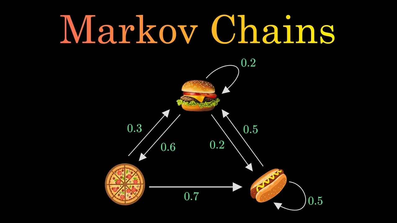
Introduction to Markov Chains: Basic knowledge of state transitions, transition matrices, and the concept of a stationary distribution.
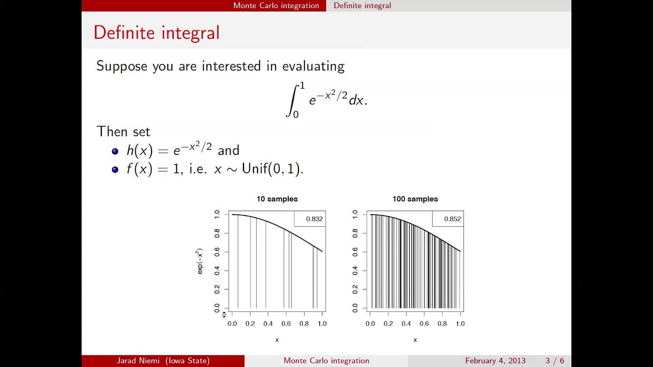
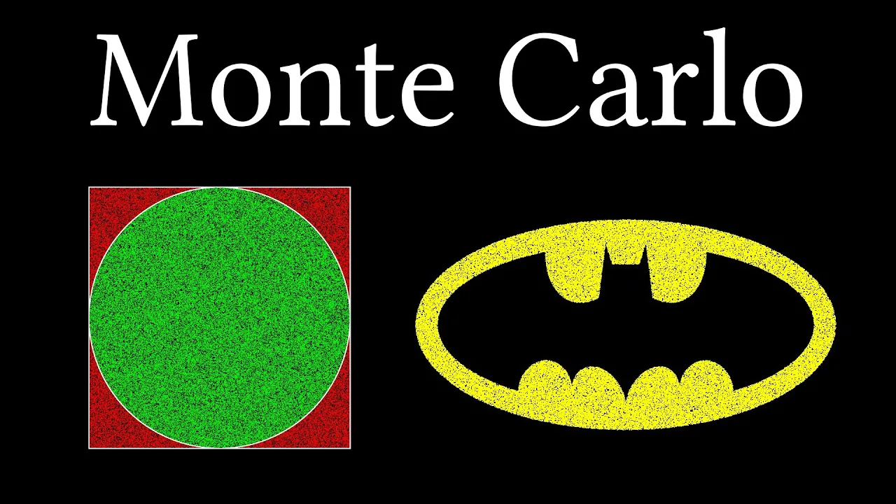
Monte Carlo Integration: The foundational concept of using random sampling to numerically approximate complex mathematical integrals.
Gibbs Sampling: Exploring a special, highly efficient case of the Metropolis-Hastings algorithm used for multi-dimensional target distributions.
MCMC Convergence Diagnostics: Learning how to assess if a chain has converged using tools like trace plots, autocorrelation, burn-in periods, and the Gelman-Rubin (R-hat) statistic.
Hamiltonian Monte Carlo (HMC) and NUTS: Advanced MCMC algorithms that leverage gradient information to sample much more efficiently in high-dimensional spaces.
Probabilistic Programming: Implementing MCMC algorithms in practice using modern computational frameworks like PyMC, Stan, or JAX for Bayesian data analysis.
86.8K views589likes10:41Original Release: 2013-03-03
hello this is Jared nimi with a mini lecture on the Metropolis Hastings algorithm previously we've talked about a desire to sample from a particular distribution whose density is f and we mentioned a few different methods that we could use to sample from this distribution the first is that if f is a known density we can typically uh simulate it directly using statistical software if it's not and we can find its CDF and the inverse of its CDF then we can sample using the inverse CDF method and finally we talked about the accept reject method where we have a proposal distribution we create an envelope around this target density F all right so if we cannot use one of these methods uh but we can at least evaluate f ofx up to a normalizing constant then we can use What's called the Metropolis Hastings algorithm without further Ado we'll introduce the Metropolis hings algorithm so f ofx is going to be our Target density and this could be unnormalized we're going to assume that we have a current value uh XJ we'll see where that comes up in a second and we have a proposal distribution that now might depend on our current value XJ all right so the algorithm then says okay the first thing we do is we sample a proposed value xar from our proposal distribution that may depend on the current value XJ the next thing we do is calculate What's called the acceptance probability first we'll start with the term on the right side here where here we have the ratio of the target density for the proposed value versus the current value and then we multiply that by the ratio of these proposal density values where here in the denominator we have the proposal draw that we actually did so that is How likely was the proposed value given our current state and in the numerator we reverse that and we say how How likely would the current value have been if we were currently at the proposed value all right so the key here is that we just have to evaluate this ratio of Target densities and this ratio of proposal densities so we calculate that value we take the minimum of that value and one this just ensures that our probability is a number between 0 one and we call that number the acceptance probability of moving from our current value XJ to a proposed value xar so we're going to go ahead and accept the proposed value with that probability so in this case we're going to set the new value XJ + 1 to the proposed value X star with that probability and if we do not accept it we're going to go ahead and set the the next value to the current value this is very important and differs from the accept reject algorithm where we would just repeat the entire process here we do not repeat the entire process we just set the next value equal to the current value all right so I want to make a couple of notes about this algorithm the first is that under certain regularity conditions the sequence of random variables XJ converges in distribution to capital X or X has the density f right so in the limit as we do as J goes to Infinity we know that we're drawing from the density F but hopefully it's clear here that the sequence XJ is not independent this again is unlike our previous methods in particular unlike accept reject the xjs are not independent because they can depend both in the proposal on the previous value and they depend via the acceptance probability on the previous value so this sequence XJ is not independent but nonetheless under regularity conditions we have a law of large numbers and the central limit theorem that says that allows us to calculate the same Monte Carlo approximation to the integrals that we've been talking about so we can take our sequence XJ evaluate the function H take the average overall of those values and that converges to this expectation that we've been interested in which can be written as this integral all right so that's the algorithm I want to give a couple of particular examples the first is known as the random walk Metropolis algorithm and this is the algorithm as originally presented by metropolis and the idea here is that you have a proposal that's called symmetric so it's symmetric if the probability moving from XJ to X and the probability of going from X to XJ is equal for all X and XJ this proposal is called symmetric and it's convenient in the Metropolis Hastings algorithm because in our acceptance probability calculation we have this ratio right here of proposal densities but by being symmetric those proposal densities cancel each other out and that part just becomes one and our Metropolis Hastings acceptance probability becomes easier to calculate because now it is simply just the ratio of the proposed value to the current value all right so notice that this means that if the proposed value has a higher density under uh the target distribution then the current value does we will always accept it and if it doesn't then we will accept it with some probability all right so I'm going to consider an example now where we've we've considered this example before here's a truncated normal the untruncated normal has a mean of five and a variance of nine but now we've truncated to be between 1 and six and we're interested in drawing samples from this distribution we've shown before we could use this to draw samples using the inverse CDF method uh but now we're going to go ahead and use this random walk Metropolis Method All right so here is our unnormalized uh Target density and we're going to choose a random walk Metropolis where the proposal distribution is just a normal distribution that is centered at the current value and has a variance of one to start the whole chain off we need to have an initial value in this case we're just going to have an initial value of five all right so we go ahead and run this random walk metropolis and we get something that looks like this all right so the key part here is the top left figure shows a bit about how the samples how this chain uh these values XJ xj+ 1 XJ plus2 are not independent right here in particular here at the end we sort of get stuck at low values in that chain um as we get more and more iterations it's harder and harder to see that they're not independent but in fact they are not independent in the bottom row here we have a sequence of or we have a histograms of the samples that we actually Drew along with the curve of the True Value right this is the true uh now normalized density for this truncated normal and we can see that with only 100 iterations with this example we don't do a very good job of approximating this density but as we gather more and more samples we do a better and better job of approximating the Target distribution of Interest all right so the second type of specific Metropolis Hastings algorithm that I'm going to mention is called is using an independent proposal so now the proposal distribution does not depend on what our current value is right so we're going to call this independent and in our Metropolis Hastings acceptance probability the P the key piece that will differ is the piece right here we now we still have this ratio of Target densities but now we have the ratio of The Proposal density as well which do not depend on any previous value because our proposal is independent we're going to continue with the example we had before and now we're going to choose as our proposed distribution here this normal with mean three and variance one all right so looking at similar pictures um we can see uh here in this particular example uh we got stuck at a particular high value for quite a long time uh as we get more and more iterations that Val that getting stuck is harder and harder to see but just like we saw before at with fairly low numbers heating the target distribution of interest but as we get more and more samples we seem to be doing a better and better job so at this point no effort was made whatsoever in these examples to uh provide a good performing algorithm they would just examples shown that the algorithm uh does in fact seem to work all right so in summary this Metropolis Hastings algorithm can be used to draw samples from a target distribution um particularly you want to think about it when other methods don't work well as mentioned this method does not provide independent samples whereas the inverse CDF and the accept reject algorithm will provide independent samples so it's often better if you can to produce independent samples and so you should try those other methods first but if you can't get those to work then this Metropolis tting algorithm uh would be the way to go um all we need to know is we need to be able to evaluate the target density up to a normalizing constant and we need to uh choose a proposal distribution but unlike the accept reject method here we do not need to find a value m that envelopes the target distribution uh based on this particular proposal distribution so that's one advantage of using the Metropolis Hastings as opposed to the accept reject all right thanks
Up Next
18:58
Gibbs Sampling Explained: A Practical Introduction with Examples
@SpartacanUsuals
86.1K views•2018-05-15

4:43
Elliptic Curve Cryptography Explained: ECC, ECDSA, ECDH
@PracticalNetworking
28.5K views•2024-10-21

8:38
Gibbs Sampling Explained: Conditional Distributions for Bayesian Inference
@jaradniemi
112.2K views•2013-03-03

6:00
The Mathematical Impossibility of Accurate World Maps
@Vox
23.3M views•2016-12-02
Related Study Plans & Knowledge Roadmaps
Structured learning paths in Mathematics
mathematics
Tensor Calculus: Vectors to Riemann Curvature
01Mathematical Foundations: Linear Algebra & Calculus
02Covectors, Dual Spaces, and Tensor Basics
03The Metric Tensor and Index Gymnastics
+ 2 more learning modules
40h5 modules
Explore Roadmap
mathematics
Gödel's Incompleteness: Logic, Proofs & Limits
01Introduction to Formal Systems & Hilbert's Dream
02Set Theory, Cardinality, and Cantor's Diagonal Argument
03Arithmetization and Gödel Numbering
+ 2 more learning modules
14h5 modules
Explore Roadmap
mathematics
Galois Theory: Fields, Groups & Solvability
01Foundations of Abstract Algebra: Groups & Fields
02Polynomials & Field Extensions
03Splitting Fields & Symmetries
+ 2 more learning modules
24h5 modules
Explore Roadmap
mathematics
Non-Euclidean Geometry: Models & Geodesics
01Euclid's Fifth Postulate and the Birth of New Geometries
02Hyperbolic Space and the Poincaré Disk Model
03Geodesics: Defining Straight Lines in Curved Spaces
+ 2 more learning modules
15h5 modules
Explore Roadmap