




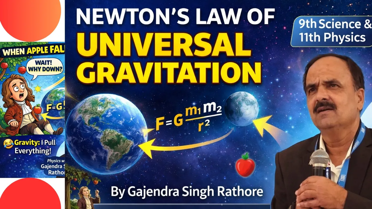

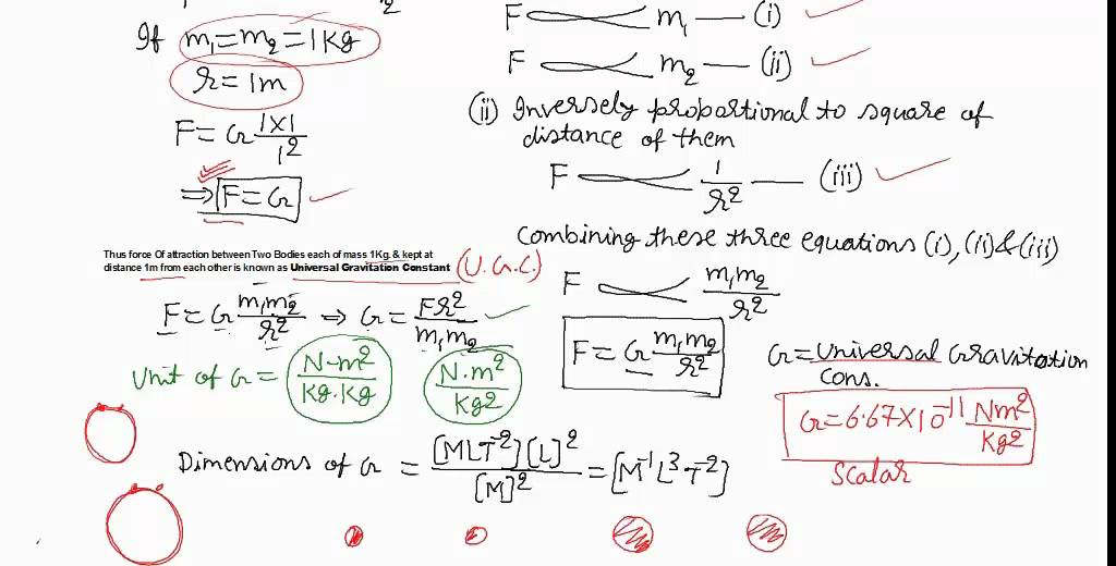





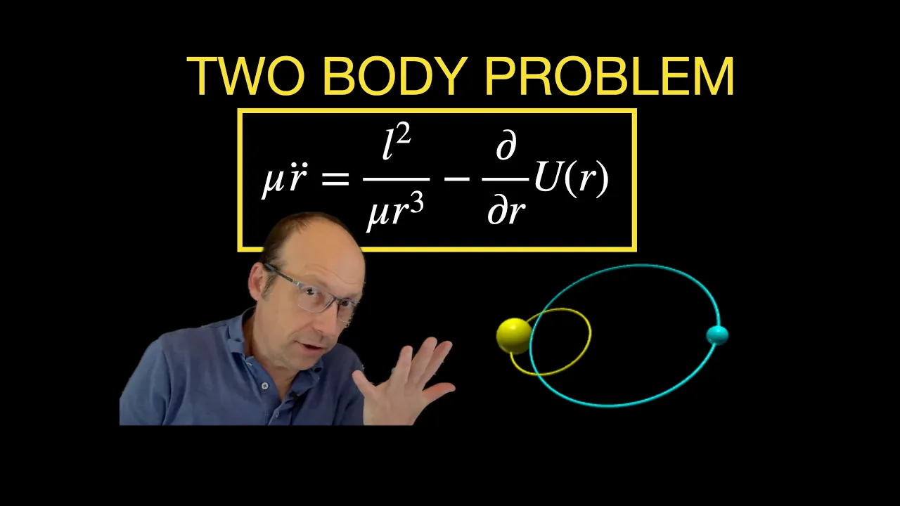
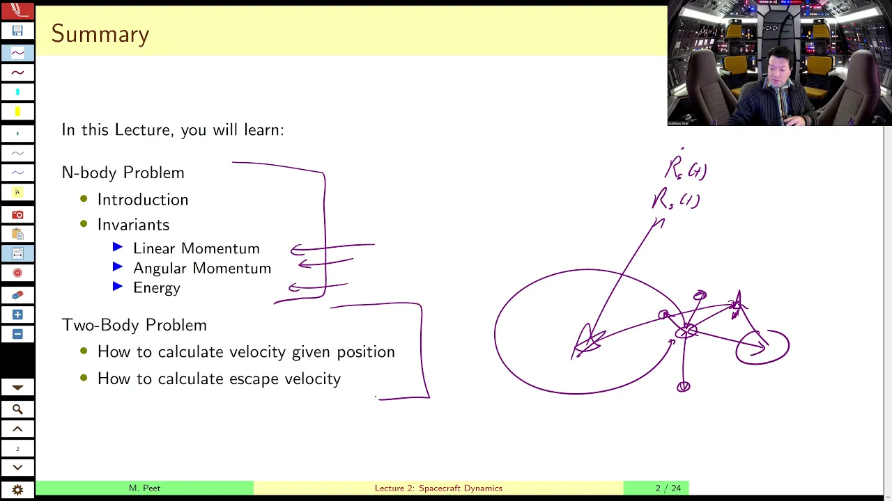












Newton's Law of Gravitation states that two point masses attract each other with a force proportional to the product of their masses and inversely proportional to the square of the distance between them, expressed as F = G*M1*M2/R². In astrodynamics, this law is extended to spherical bodies and expressed in vector form as r̈ = -μ*r/r³, where μ = G*M is the gravitational parameter. This equation describes the relative acceleration of a spacecraft with respect to a planet and forms the foundation for analyzing Keplerian orbits. The gravitational forces are conservative, meaning mechanical energy is conserved, and the center of mass of the system moves at constant velocity.
Newton's Law of Gravitation | Astrodynamics Lecture 4
Added:Newton's Three Laws of Motion, particularly the relationships between force, mass, and acceleration.
Vector algebra, including position vectors, vector subtraction, unit vectors, and vector notation in three-dimensional space.
The scalar representation of Newton's Law of Universal Gravitation and the concept of the gravitational constant (G).
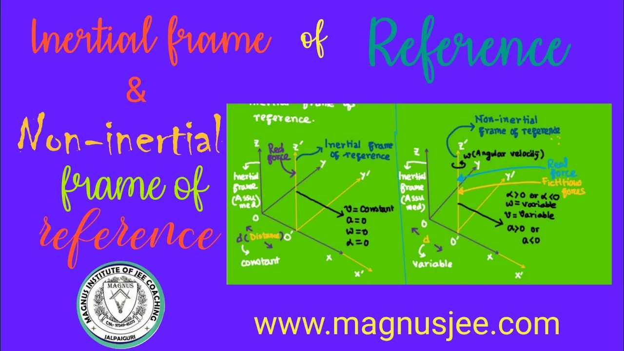
Basic kinematics, specifically relative position and the concept of inertial versus non-inertial reference frames.
Formulating and solving the Classical Two-Body Problem to determine the relative motion of two orbiting bodies.
Deriving Kepler's Laws of Planetary Motion from Newton's laws, and understanding conic sections (circular, elliptic, parabolic, and hyperbolic orbits).
Defining orbital state vectors (position and velocity) and converting them into Keplerian orbital elements.
Exploring orbital perturbations, such as atmospheric drag and planetary oblateness (the J2 effect), which cause deviations from ideal Newtonian orbits.
605 views5likes51:01Original Release: 2017-01-11
running all right okay everyone few things before we actually start Newton's gravitational law and actual astrodynamics so I made a mistake last time in computing the acceleration of Q so solving this problem everything was correct up until the end when I was rushing it and I missed the piece and thanks to whoever pointed that out so the velocity of Q with respect to the ground which is inertial well that that was right - our alpha dot sine of alpha X let's see plus R alpha dot cosine of alpha ey in the next step I just ignored one piece in the product rule for derivatives so these are two functions alpha dot and sine a lot for the depend on time so I was missing one of them and in particular this one so if you take the rate of change of these it's minus R alpha double dot sine of alpha and then minus R alpha dot squared cosine of alpha e^x so I was believed I was missing this piece plus same story there are alpha double dot sine of alpha minus R alpha dot squared I'm sorry this remains the cosine alpha double dot cosine alpha then minus R alpha dot squared sine of alpha D Y so I believe I was missing this piece so your astrodynamics professor cannot take time derivatives when he's not paying attention that's what happens so sorry about that thanks for pointing this out that means someone is paying attention all right everything else was correct so I hope you guys went home and tried to finish these and also solve it without the angular momentum approach and see how much more difficult it could be any questions about everything that we done up to this point it's pretty known stuff right a couple more announcements before I start I don't have office hours today I have a personal confident I have to run away but I will have them on Friday right after class for an hour or so so sorry about that is just for this week and I did post I posted on the calendar for this class and also sent an announcement the last week of this month I won't be here I'll be on travel and so 23rd 25th and 27th I think those are the days where we would have lectures I will give you old videos to cover the topic so we don't fall behind if that's okay with everybody I think the homework is the week after that so we'll we'll meet again before the homework anyways okay I'll leave it up for a second here so today we will start real astrodynamics Newton's law of gravitation I'll go through a few things few definitions and properties so given two masses two particles point masses M 1 and M 2 this is how its stated at the beginning so two points with mass M 1 and M 2 the let's start with a scalar expression the attraction that they experience due to gravitational force is given at least in its norm by G m1 m2 over the distance between the two let's call it R squared where I have this constant here I just happened to write it down but it's it's in your book where the gravitational constant is this value here which you're more than welcome to memorize or just know that you have to look it up in the book when it's needed ok so these are two point masses they're attract each other with this force and I'm just talking about the magnitude of the force for now given the ten to the minus eleven here those masses who have a measurable attraction have to be pretty big so two people they can attract each other for other reasons but not for that there will be so weak that we cannot measure it if you're talking about the few hundred pounds you really need several thousands of tons to have something measurable in particular as you can imagine at some point we'll say that for example M 1 is the mass of our planet and these is also something we'll will show if we have time today I'll start opening MATLAB if not we'll do next time but I have the constants in an example I think this is in the order of 10 to the 24th kilograms it's a pretty big value and then m2 will become just little m a spacecraft and so in general we'll have the condition where mass of the planet is much bigger than middle m and why am i saying that even if it should be obvious it's because I usually get the question at this point what if I'm talking about several tons the International Space Station your station has to be pretty big until you get something noticeable in terms of not neglecting little m so it's usually the case that that's that's the mass of the plant is much bigger than your spacecraft unless you're looking at the moon which is not an artificial satellite of course so what happens if we're looking at this situation here well if you divide times M 2 which would be your object attracted by the planet you have the gravitational acceleration and again I'm still talking about scalars here what we call G can be expressed as G the gravitational constant the big G times mass of the planet over R squared which I can rewrite if we assume as we'll do at the beginning that the planet is a sphere is radius of the planet plus altitude over the surface squared and what have I just done here that contradicts what I just told you the beginning remember I said Newton's law of gravitation starts with two point masses right they attract each other with this force etc accelerated is the constant what have I done here that contradicts my initial statement yeah but that's okay because that was a force and this is an acceleration so I can do that so it doesn't contradict my initial assumption but by saying that I'm talking about my planet I am NOT talking about point masses anymore this planet is big it's not a point mass anymore but you can still do it we're not going to demonstrate it but the demonstration is pretty straightforward it's not in the appendix of your book these law of gravitation is still valid if your point masses are actually spheres and so perfect spheres so this is for example m1 and this is m2 and and the mass inside the volumes are it's distributed in a uniform way so for example say this is your planet and these collapses to really just a point because it's very tiny you can imagine how you can get still an expression like this because you're going to say that each individual infinitesimal mass that composes m1 DM is going to attract m2 down here with the force that looks like this but then you always have the symmetric one down here so you go over a volume integral and at the end of the day you're going to get this exact same expression it's in the appendix of your book but def that law works for point masses and also for spherical uniformly distributed mass type of objects okay which is what we have when we look at our planet in first approximation and a spacecraft so that's why I can say these I can look at an actual sphere and of course these should collapse into G 0 which is 9.81 meters over seconds squared the usual value that we use when we say that we are at the surface so if you're taking the values mass of the earth again I do not recall the exact value this is usually six thousand three hundred and seventy eight kilometers average radius of the planet again we'll see all these numbers once we start playing with MATLAB and solving actual numerical problems but that's that's what we have scalar wise but we're doing dynamics so we better talk about vectors here so let's see how we express the gravitational force in three dimensions so basically I'm going to redraw something that we have seen already two reference frames at some point will be two reference frame let's start from the first one the usual inertial one that has an origin at O and then I have my two masses m1 and m2 let's say that m1 is here and it's position is given by vector R 1 and M 2 is here its position is given by vector R 2 and I'm going to call the vector originating from m1 going to M 2 basically the position of M 2 to respect to M 1 little odd and maybe also called the unit vector that goes from m1 to m2 just the direction little UI well what we said in vector form will look like this the force that must one experiences because of the attraction from mass 2 is G M 1 M 2 this should not be new stuff by the way it's probably not new stuff for you but and this is also equal to M 1 R 1 double dot I am assuming from this point on that when I put a dot on top of the vector that's its inertial time derivative in other words I will assume this that when I stake a vector B and I put a dot on top of it this is the rate of change of the vector taken by an inertial observer so this is inertia okay so that's Newton's second law this is the force the model of the force this is mass times acceleration and the same for the other one except that is the third law of Newton which is action reaction so there must be a - it's the same force except it's pointing the other way so this is what I have this is m2 r2 double dot you've probably seen this stuff somewhere I think so a few fun facts about these force or forces first one is you can easily prove that wherever the center of mass of this system of two particles is it's moving at constant velocity with respect to the inertial observer so it's it's acceleration is zero so let's just say that it's here so in this sketch is like saying that m2 is a little heavier than m1 but I will actually say at some point at least the planet but it doesn't matter so what is the acceleration of G of the center of mass with respect to n how would you compute that I have the acceleration of them one right it's this one divide it so look at these equality right here right R 1 double dot is the acceleration of m1 if I divided by m1 I get its acceleration but what is the definition of acceleration of center of mass for the system of particles you have to do summation over all the particles of M I the acceleration of all the particles and divided by the sum of all the particles all the masses right it's a it's a weighted average right so this case is just two of them so it's going to be M 1 R 1 double dot plus M 2 R 2 double dot divided by M 1 plus M 2 which you can easily see because it is minus that this is zero vector interesting fact center of mass does not accelerate translates constant velocity okay that's one thing the second property which is probably more interesting and we'll definitely use it quite a bit is that what kind of forces are these gravitational forces they have a very important property similar to spring conservative forces yes these are conservative forces and so again this is dynamics material that you should know but for what we care in this class these means so conservative that for example if I define the mechanical energies as the kinetic energy plus some potential energy for each of the masses it's a scalar value that it's constant in time once we define orbital parameters this mechanical energy for a given orbit will be a function of the semi-major axis of the orbit so there are some geometrical properties of all bits that have to they connect directly to the mechanical energy so there are very useful relationships that we'll be able to derive so but that's a fact when you have conservative forces and and what is V for this type of force this V will prove it if you want is this scalar potential energy function G m1 m2 over R remember little R is the distance between the two all right I asked you a question how do you prove that this is in fact a potential function that you can use to obtain the forces what would you do what happens if you have a conservative force and you're given a potential function what can you do with that function other than stick it in here and say that T plus B is constant okay that's fine we've done that conservative forces do work that I'm sorry that is the potential energy function I want to use it so when you're given a potential energy function you can camp T in the force and that's the property of being conservative and the fact that work done does not depend on the path again go back to your from dynamics book but what we need to know is simply this that f of G so for example f12 in particular I can get it from these by computing the gradient with a minus in front over the radius of the scalar function V remember this thing you probably haven't used it very much but it's it's one property of conservative forces why am I going to prove this to you and show it here it will become clear when we'll talk about all the tall perturbations and the fact that the planet is not an actual sphere because there are more complicated expressions for potential functions with morte here that allow you to model different shapes this is good for a spherical planet so how do you compute that any ideas so say that little R that vector that goes from act m1 to m2 is projected in these bases attached to the inertial frame let's give this unit directions names I J and K why not can call them that way it's three axis right so say that I call the unit directions those ways I can I can write this right agree I just called little X little Y little Z the projections of our on those three directions well then that gradient the gradient over R of V is defined as the partial of V with respect to X I plus the partial of V with respect to Y J plus the partial of V with respect to Z K I know it doesn't seem very useful now but it will become useful in the weeks to come so let's let's do it but I need one more step how do I take the partial for example V with respect to X what would you do Vee is this expression right here right forget about additional potential terms that's B I need to find a way to take the partials partial derivatives of that scalar function with respect to those three coordinates XY and Z what is the first thing that you want to do maybe yeah are these already expressed in terms of XY and z the vector so just the scaler so basically I might say okay if I'm using those coordinates this is G m1 m2 that is multiplying x squared plus y squared plus Z squared to the minus 1 over 2 right just another way to write square root at denominator there's a minus here okay so now I can take the partial of these so it's going to look like these the partial of V with respect to X let's see minus 1 over 2 goes in front - goes away 1 / - those are constants m1 m2 these remains x squared plus y squared plus Z squared now it's minus 3 over 2 and then 2x I'm not going to pause here because it's another derivative and I want to make sure that I have paid attention this time I think it's correct okay well this is x I okay and you will have very similar terms for the other ones and 1 and 2 just let's say whatever it's in here - 3 / - it's the same parenthesis now here you have a - y g+ + similar or similar except here you have 2 z k few simplifications of course what happens well what happens is that you have this G m1 m2 over this square root of these cubed right we see that that I can collect do we do that okay and then the vector parts basically become XY plus YJ plus ZK which is nothing else than the R vector and so I just going to bring everything here I claim that I could get f1 2 as minus the gradient over R of V which is what I just computed except I don't have the - there but but that's what I have I have minus G m1 m2 that square root cubed at the nominator is basically R cubed and that is R so this is exactly this force up here if you multiply numerator and the numerator times R that that's that's what you get agree so these are not things that I I want you to be able to do right away but you need to know that they exist and you need to know what page of the aerodynamics book - you need to open - whoa ok potential function this is what I have to do these are the steps I can get a force I also have to refresh it myself I don't go around thinking about potential functions every day of the year but when I need them I know where they are so these all interesting stuff that we use here and there but I haven't done the very interesting thing that I want to do today yet ok which page can I erase I think I think this one so only this before I move on just a suggestion I wrote down here at page 66 of your book since again we're very close to using MATLAB for the first time there are a couple of your book the third version at least I don't know about the second version but the version I have and I put in the syllabus has appendices with MATLAB code and there is a toolbar 3d Dot em file and a three body I think yes dot M file that I invite you to play with they're just there for you to use I think when you buy the electronic version you can download m-files I think that's what I've done years ago what's your years ago so these all these things that I'm telling you do these finish this at home they're basically uncollected homeworks the idea is that there will be a seamless transition to homeworks and tests so that there's no surprises other than those you create for yourself so do do this it's gonna take a few minutes it's cold that it's ready for you you can play with it until I'll show you the code that I will share with you next time or this time if we can make it but yeah do that but now what do you think we really care about what we care about is the situation where this is going to be my planet Earth for example and this is a space artificial satellite so I don't really care too much about what the inertial observer can see because I cannot be this guy probably I cannot be these little men here sitting on the Sun remember the problem we solved last time in 2d I'm going to try to see if I can do the same now in 3d basically if I can look at these Verity motions that is given by this little R vector from this point of view and and and basically see the same thing that the inertial observer sees without being the inertial observer because that's what happens we're sitting on this part on this planet we launched a satellite we can measure what it is from here we're not going to the Sun and measuring bigger one and big R 2 and then subtract we cannot do that right so what I'm saying is that I care basically about this vector acceleration of R 2 we respect to R 1 right but this is still taking all this time derivatives are taken by n ok this is this is all and sees the relative position of m2 respect on one changing in time okay that's a fact so well we want to analyze these these are double dot and let's actually write it what is this going to look like is the following if you go back to what I just erased you're going to be left with minus G m1 plus m2 over say R cubed R again go back to what I just erased basically take the force that is acting on mass 2 divided by little m2 and the same for this divided by a little m1 and you get the accelerations subtract this is what you have this quantity here is called the gravitational parameter it changes depending on the masses m1 and m2 for the earth is obviously I don't have the medical number here written down for you but it's again known constants in the books actually let me I just used Big M right so for for our planet is what you have g m-e why because if this is the planet and this is a satellite I do not care a big this International Space Station can get it's going to be tiny compared to the mass of the planet so we just say it's GMP you can you can do this exercise and see how how much difference it makes to have a ton ten times thousand tons of em - it's it's makes no difference so this is a constant okay so in other words the acceleration the relative acceleration of m2 the acceleration of M to respect someone as measured by endo for now is given by this model minus mu over R cubed R which is the same expression I had in the XS last time right that dynamics problem we were solving that I projected so this is the starting point of astrodynamics this is the model of acceleration and we still have to say a few things about this that will bring to the ability to describe different shapes of orbits Keplerian orbits they're called capillary after Kepler and this is only assuming a perfectly spherical planet because that's where I started from at some point during the semester we'll add plus other terms to model more realistic shapes for the planet but we don't do it for now as a matter of fact in the MATLAB code the first MATLAB code that I want to show you I will integrate this equation numerically and I also have an extended expression that takes into account the oblate Ness of the planet basically the fact that the planet is not really a sphere but in first approximation you can make it an ellipsoid where this is North Pole and this is South Pole so it's it's like new squeezing at the poles we know that that's the shape we have plus other bumps but there is an expression here you can add to add what is called the j2 effect we'll talk about this I'm going ahead myself but I will show you how much of a difference he makes to have this term or not for all bits like the one of the International Space Station low-earth orbits where you're close to the planet ignoring the effect of the oblate Ness at the poles means that you basically ignoring what it's actually happening your orbit is not frozen in time is continuously changing changing playing changing orientation in space oscillating on the shape so that's reality and so not having that those additional terms means that you're basically doing baby astrodynamics which is most of astronauts classes do to be honest but I stress on the perturbations because that's that's what you really need to use so we'll see that in MATLAB but we start from this model everything is perfect everything is spherical capillary on orbits now this is what this is a second order of course differential equation vector differential equation and how many so if you want to integrate this in time it doesn't have an actual analytical solution but it doesn't matter analytically or numerically what do you need to integrate the second order differential equation that is actually a vector differential equation what would you need what do you need to integrate a differential equation if I thought I'm going five if I'm telling you that I'm going I'm traveling at five meters per second constant speed and I ask you what am I going to be in five minutes the initial condition right wait were you starting from I mean it's I don't know where you gonna be in five minutes if you don't tell me you're starting points right starting point so how many initial conditions do you need hey go higher more 6y6 because that's a second-order differential equation if you add a simple differential equation scalar differential equation I don't know X double dot equals KX you wanna integrate these you need X at time zero and X dot times zero because that's second time derivative right you need to know those are three equations because that's a vector in other words let me write it here if I want to write the scalar form of these this is what I have remember how I defined R I have X double dot which is equal to minus mu over the square root of x squared plus y squared plus Z squared cubed times X then same story for y so basically here I have the same times y and then for Z I have minus this expression times Z so now these has become three scalar differential equations of the second order so for each one to new traditions basically if you want to count it that way so you need six you need an initial condition in XY and Z you need to know initial relative position and you need to know initial relative velocity for example so that you can solve these differential equations make sense by the way there are no linear differential equations if my body balls are XY and Z it's obviously nonlinear square roots cube etc etc so nonlinear what does it mean integrating in time it means that you start from this position and velocity and you can have a time history for X Y Z X dot y dot 0 you can plot a trajectory in 3d you can tell me what the velocity is at a given time a position at the given time that's what it means solving the differential equation ok now these are not the only constants that you can use these are the obvious ones because I'm working next y&z when we talk about orbital parameters not too far from today we'll see that there are much more user-friendly constants of integration that you can use there are not XYZ X dot y dot Z dot we don't really look at satellites that way there are all little quantities properties of of conics that we can use as constants of integration but for now that's what we have ok now I wrote this and again this is the time derivative of this are vector taken by this observer but I am NOT Here I am up there I am on the planet can I still claim that what I see is equal to these yes if you choose your reference frame wisely so I am going to basically resolve the same exercise we solve last time in 2d I just do it in 3d remember what we did at some point we derive an expression or Monsieur I don't wanna that's right here we said okay I have an observer a I have an observer B I have a point P and we found an acceleration relationship right remember that so I'm going to do the following now this a becomes n these P becomes M 2 and this B is my planet M 1 so basically I'm saying K I'm going to choose a reference frame now whose origin of the coordinate system has the origin at M 1 right here and I don't know anything about the orientation for now just leave it free to change but I do know that that reference frame contains M 1 which is the planet ok maybe a reference frame for now is the planet so it actually rotates with the planet so if you go back to last lecture at the beginning and you take that acceleration relationship and you substitute where you see a you substitute n where you see B is substitute M 1 where you see P you substitute M 2 this is what you get and I told you I don't memorize that expression in fact over here the acceleration of the mass M 2 seen by the inertial observer is equal to the acceleration of the mass M 2 seen by M 1 plus the acceleration of m1 seen by the inertial observer plus 2 Omega of M 1 with respect to n I know you're thinking these was a point and you're telling me that this is the angular velocity of the point with respect to n no I am saying that this is a planet and for now I am using the planet as a reference frame so the origin of the coordinate system in their reference frame is m1 but there is an actual reference frame the rigid body moving around the center of it is m1 what was i okay cross with the velocity or them - we respect to m1 plus more terms alpha and you know acceleration of m1 with respect to n which is crossing our m2 with respect when one last term Omega M 1 with respect to n which is crossing another Omega of M one respect when crossed with the same our m2 to respect to m1 do you have any questions at this point is this clear what I'm doing I am doing exactly what I've done last time reference frame a reference frame B I'm looking at a point except I'm changing the names I'm saying that a is my inertial observer B is an observer that he's attached to the planet and one and and and the point that I'm looking at is my spacecraft m2 so it's the same expression we derived last time I just changed the the name of the superscripts and subscripts yes m1 sorry yes so let's let's refresh it this is the acceleration of the satellite m2 seen by the inertial observer this is the acceleration of the satellite seen by the planet me sitting on this planet m1 this is the acceleration of the planet seen by the inertial observer this is what we call the Coriolis acceleration if you want the cross product of Omega and the relative velocity this is the term due to the relative angular acceleration and this is what usually is called the centripetal piece so this m1 is supposed to be on top of this omega okay all right so look at the what I have here what is if I take this term and I bring it to the left acceleration of m2 respect to end - acceleration of m1 with respect when this is equal to the acceleration of m2 with respect to M one plus I'm going I'm not going to write all these terms basically here I have a bunch of other terms this ones that have either Omega or alpha in them right yes can you cross a scalar with something okay so that's that's a scalar that is multiplying a vector yeah you first do this cross-product then you just multiply times to whatever vector comes out of these you just make it twice yep is this clear I just taken this piece moved it here and then the rest is the same so I have this one am to respect term 1 plus all these other terms what is these see that I called it there big R 2 double dot and big R 1 double dot but that's what they are this this is this is the acceleration of the second mass with respect to the inertial observer that I called that way and this is the acceleration of the mass m1 respect to the inertial observer that I called that way right and so this is little R double dot so little R double dot is actually equal to the acceleration of m2 seen by m1 plus all these other stuff ok and all these other stuff again contains omegas and alphas or few omegas and 1 alpha but angular quantities quantities that tell me that the frame appear that I've chosen is changing orientation maybe changing orientation respect away or n in this case what if I pick something that doesn't change orientation with respect to N if instead of going with the planet I go with the planet but the coordinate system I chose it I choose it so that the axis for example remain constantly aligned with the axis of n so it doesn't matter what M one is doing but the axes are not changing orientation what happens here this is gone no more Omega no more alpha right so if I assume that I have an observer sitting on the planet and I choose my coordinate system so that the that it's not rotating with respect to the inertial observer which is what I call DCI last time I've just done it in 2d remember that plan we did last time I had two axes on the Sun and the same two axes on the earth I'm just doing it in 3d so if I see it on the planet and I choose the coordinate system doesn't change orientation with time then I can claim this and this is very important because this is telling me that it's OK for me to sit on the planet even though it's not an inertial point of view because the acceleration that I measure from here for the satellite which is M - it's it's R double dot it's the actual relative acceleration that an inertial observer would see so I can basically use everything that I've done by measuring this because in practice I know if this is something you can appreciate mathematically speaking but in practice we measure this stuff here we can measure things from here from m1 not from somewhere else no question does it make sense so in other words from now on I'm going to work with this knowing that I need that I can equate that to what I see from the planet if I choose the following situation following coordinate systems again the inertial observer here planet Earth now I'm not gonna call it m1 anymore you choose your axis so that they can be parallel to this they don't have to be parallel to these they just don't have they can't rotate they have to be a zero angular rate and angular acceleration make sense so if I choose it this way what I call the last time is CI then whatever I'm measuring from here whatever these little are vector is doing that is going to my spacecraft whatever I measure from here it's equivalent from what the inertial observer is is measuring so I can now sit on the planet and be confident that I can use this expression here make sense otherwise I could not do it yes the Sun or it doesn't have to be the Sun yeah but if you want to connect it to the problem we saw the last time yes it could be the Sun when it will be time I will more formally define ECI as a reference frame whose coordinate has the center at the planet does not rotate with the planet these x axis is pointing to a certain constellation which is which is Aries and then there is Y ax the z axis I think it's south north and then you cross until you get the Y so there are specific directions in space that are chosen for this to basically say that it's not rotating that it's inertial and this is updated every 25 years we'll go through this when the time comes so it's not frozen forever it actually changes after decades it's gets updated so now before we yeah no MATLAB today but but I can introduce what we're going to do with MATLAB how you actually integrate this equation in MATLAB because that's what want to do next time do you have any questions is this clear you start from the law of gravitation we know you can extend it to spherical bodies we care about the relative motion because really I want to sit on M 1 this is the law that give me the differential equations I can integrate but I want to make sure that I can use it be in M 1 and that's what I've proven right there ok how do you how many so you guys have used MATLAB before right so have you used Oh de 45 and you integrated equations numerically you know we've done that no I see heads doing these and other heads doing this so just as an introduction we said that these differential equations that we have are going to look like this - me over square root of that stuff cubed x y double dot is equal to minus mu over square root of the same cube y + Z double dot is equal to minus mu square root cubed Z now when you are this is in general really for people working in dynamics and controls we try to rewrite systems of differential equations because it is really a system of differential equations so that the second time derivatives go away don't really go away you just do a substitution of variables and you make the system bigger and just dots appearing instead of double dots you basically do a state space representation by the way X Y Z X dot y dot Z dot this is what we will call the state vector so how do I make these uh Newton's where transform the system into something that doesn't have second-order time derivatives anymore you do the substitution calling for new variables say X 1 is X X 2 is Y X 3 is x4 is X dot X 5 is y dot X 6 is Z dot which is equivalent to that state vector you can call this if you want big X capital X big vector so with that substitution this system will look like the following and the reason why I'm writing it this way is because that's how MATLAB takes differential equations in and integrates them ok let's see let's look at the first equation what is X double dot it will become x4 dot right I'm gonna write it down here x4 dot is equal to minus mu now here you will have if you want to be thorough you have x1 squared plus x2 squared plus X 3 square cubed times X and X 6 X 1 X 5 dot is equal to minus the same don't make me write it again please this is X 2 and X 6 dot which is Z double dot is same quantity here X 3 right agree with that is just change of variable and then on top of these I'm going to add 4 5 6 X 1 dot is equal to what X 1 dot is X dot it's X 4 X 2 dot is what is X 5 X 3 dot is X 6 this is my new system of now six differential equations where there's no second order time derivatives just added more variables and make them disappear but at the end of the day they didn't really disappear I just increase the size of the system so this is our mantra we'll take your it will take basically this side here we'll see you next time and every time step we'll integrate it so it means that is going to generate at each time step that vector the integral of these which is X 1 X 2 X 3 X 4 X 506 and each time step will give you the state vector because that's what it is so that's how you set it up in MATLAB so that you can create at each time step position and velocity again Vladdy position ready velocity yes I'm sorry can you ask a question when I do this when I go from this to this it's the same questions yeah you don't change really anything I mean if you if you think about what you have to do here you have to integrate twice three times I integrate once six times in terms of complexity operations you really keep doing the same thing it's just it's just the way MATLAB will handle it I think we're up with time so we'll see a matter of example next time yes X 1 is X X 2 is y X 3 Z Z should be X Y Z X dot y dot Z and so when you see them with dots of course this is X dot y dot Z dot X double dot y double dot Z double dot this resin
Up Next

14:45
Impulsive Maneuvers & Co-Planar Orbital Transfers | Cornell Astrodynamics
@dsavransky
730 views•2022-05-04

12:53
21cm Hyperfine Transition in Neutral Hydrogen: Radio Astronomy Basics
@AaronRobertParsons
12.4K views•2011-10-13

32:32
NMR Spin Physics I: Zeeman Effect, Resonance Condition & Larmor Frequency
@nptel-indianinstituteofsci8064
2.3K views•2024-01-17

27:14
Entropy and the Second Law of Thermodynamics Explained
@veritasium
27.5M views•2023-07-01
Related Study Plans & Knowledge Roadmaps
Structured learning paths in Physics
physics
Nuclear Physics (Decay, Fission & Reactors)
01Atomic Structure and the Binding Force
02Radioactive Decay and Half-Life
03Nuclear Fission Mechanics and Chain Reactions
+ 2 more learning modules
12h5 modules
Explore Roadmap
physics
Soft Matter (Polymers, Colloids & Rheology)
01Foundations of Soft Matter & Thermal Forces
02Polymer Physics and Macromolecules
03Colloids, Surfactants, and Self-Assembly
+ 2 more learning modules
38h5 modules
Explore Roadmap
physics
Analytical Mechanics: Lagrangian & Hamiltonian
01Mathematical Foundations: Calculus of Variations
02From Newtonian Mechanics to Constraint Dynamics
03The Principle of Least Action & Lagrangian Mechanics
+ 3 more learning modules
28h6 modules
Explore Roadmap
physics
General Relativity (Spacetime & Cosmology)
01Foundations of Relativity: Special Relativity
02The Geometry of Spacetime: Equivalence Principle & Curvature
03Einstein's Field Equations: The Mathematics of Gravity
+ 2 more learning modules
55h5 modules
Explore Roadmap