


![10-12. [역학] 강체_오일러 각](https://i.ytimg.com/vi/BnyOq7ktCno/maxresdefault.jpg)





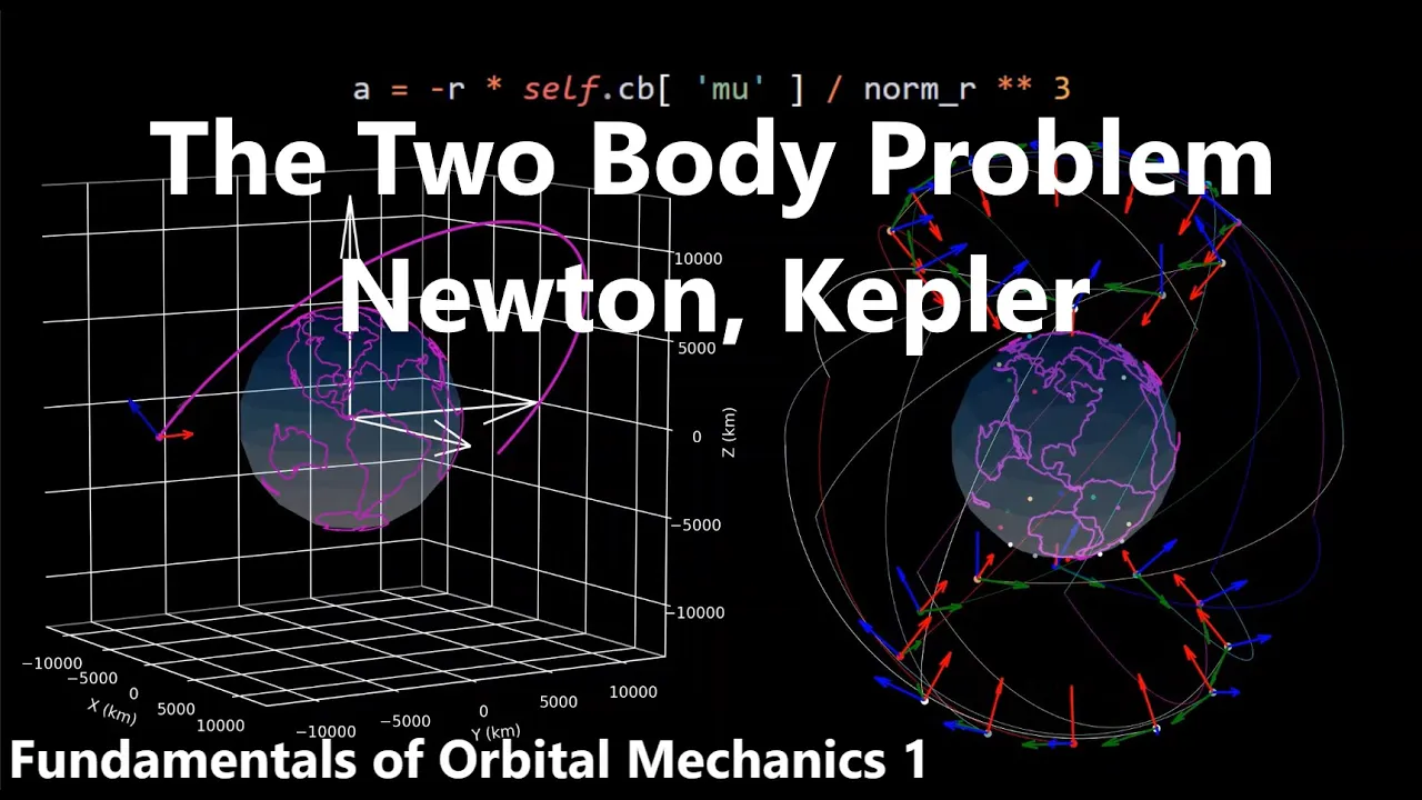




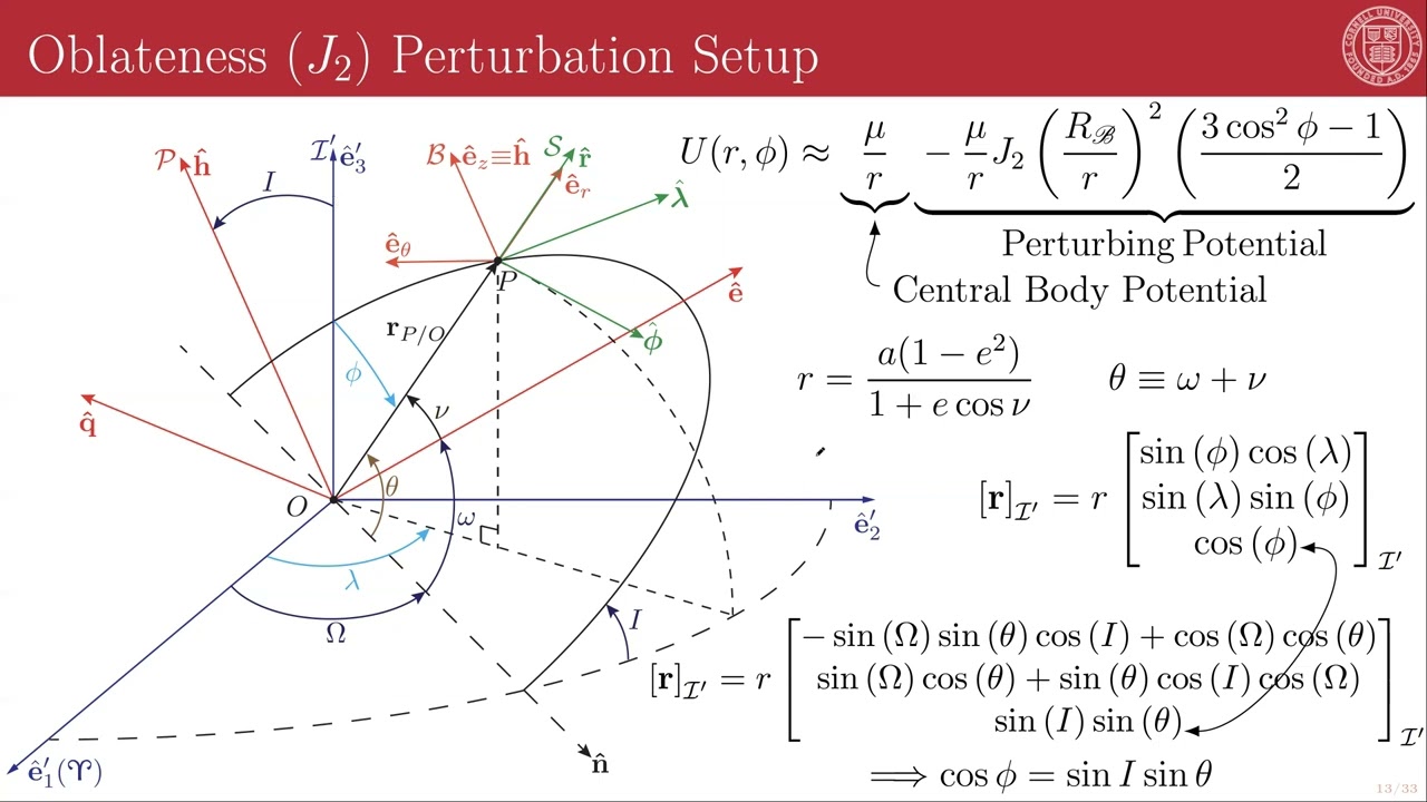



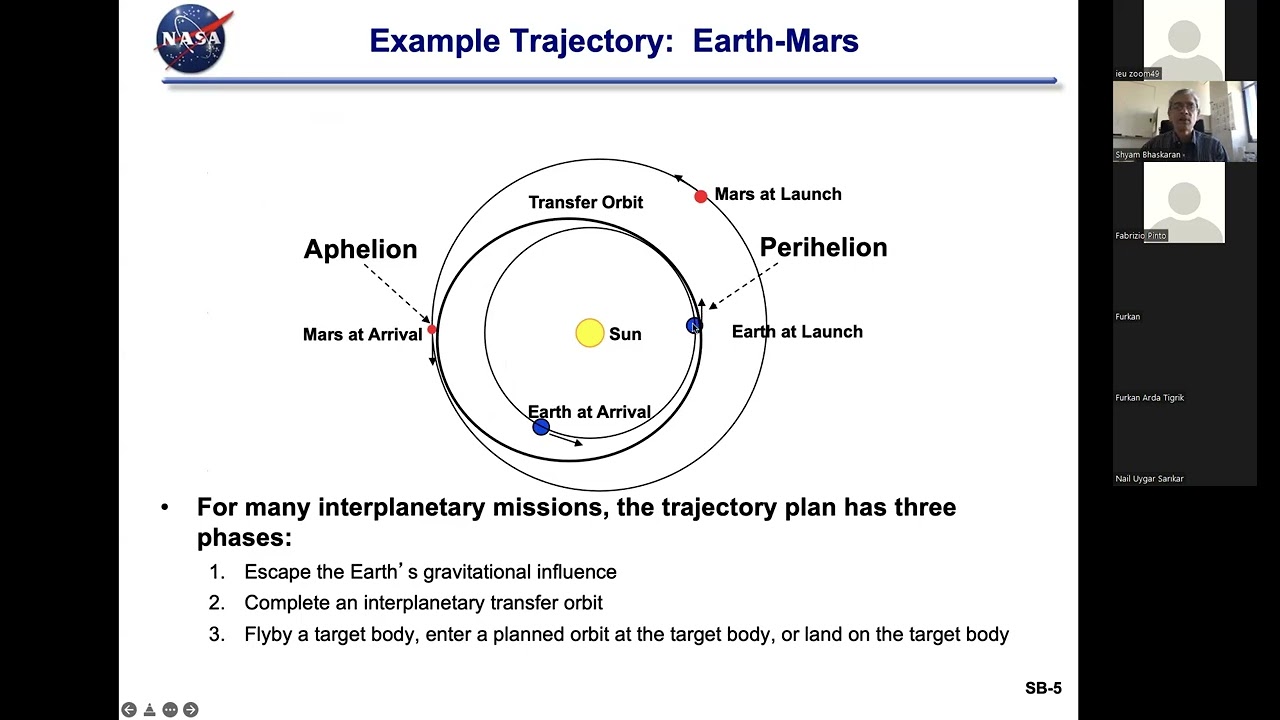

To convert orbital elements (semi-major axis a, eccentricity e, inclination i, right ascension of ascending node Ω, argument of periapsis ω, and true anomaly f) to position and velocity vectors in Earth-Centered Inertial (ECI) coordinates, we first calculate the position and velocity vectors in the perifocal coordinate system (where the x-axis points toward periapsis and the z-axis aligns with angular momentum), then apply a sequence of three rotations: R3(ω) × R1(i) × R3(Ω), where R3 represents rotation about the z-axis and R1 represents rotation about the x-axis, with the rotation angles being the argument of periapsis, inclination, and right ascension of ascending node respectively.
Orbital Elements to Position and Velocity: ECI Conversion Explained
Added:Understanding of the six classical Keplerian orbital elements (semi-major axis, eccentricity, inclination, RAAN, argument of periapsis, and true anomaly).
Foundational knowledge of linear algebra, specifically 3D rotation matrices (Euler angles) and coordinate transformations.
Familiarity with astrodynamic reference frames, particularly the Perifocal frame (PQW) and the Earth-Centered Inertial (ECI) frame.
Basic Newtonian mechanics and the two-body problem equations of motion, including how position and velocity are represented in a planar orbit.
The inverse transformation process: deriving classical Keplerian orbital elements from ECI position and velocity state vectors.
Converting ECI coordinates to Earth-Centered Earth-Fixed (ECEF) coordinates to plot ground tracks and calculate geographic coordinates.
Numerical orbit propagation and perturbation analysis, such as modeling the effects of Earth's J2 oblateness or atmospheric drag on state vectors.
Orbit determination techniques, such as utilizing observational tracking data to estimate a satellite's state vectors and predict its future path.
8.8K views95likes31:22Original Release: 2021-02-09
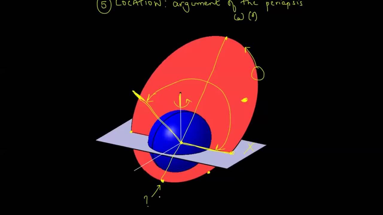
all right hello class welcome back to part c of this lecture where we get to the real meat um hopefully i've prepared you in uh part b uh with some discussion of rotation matrices for what we're about to do uh so specifically we are going to go from position and velocity vectors in satellite normal or peripheral coordinate system to eci coordinates several rotations have to take place before we get there however so uh just a rehash of what perifocal and satellite normal coordinate systems are uh so in particular the perifocal coordinate system is the coordinate system where the x hat vector is aligned with the eccentricity vector so that we have x hat pointing towards periapse the z at the z vector is pointed out of the orbital plane so aligned with the angular momentum vector this is aligned with the eccentricity vector and the y-hat vector is just given by the right-hand rule x z so y is pointing up not aligned with anything in particular so why and then of course the satellite normal coordinate system where the uh x hat vector is in the uh veloc in the position vector direction and the uh z-hat vector is also angular momentum and the y is defined by the right-hand rule somewhere over there so first we'll talk about a position vector because that's by far the easiest so in particular we have the position vector in the satellite normal coordinates which are these ones right here and that's of course right just r the radius 0 0 right because by definition the radius radial vector is aligned with the x-axis now a very simple rotation will give us the position vector in the peripheral coordinate system but it's worth the just getting it getting warmed up to do that rotation as opposed to just giving the formula here so remember of course that the radius magnitude is just given by the uh the the polar equation so i don't even need to highlight that so we've got our position in the satellite normal and we want it in the perifocal pqw frame so what is that well uh now remember what i told you that the rotation that we apply to the position in satellite normal is a is a negative of the angle that we use to get from the satellite normal to the peripheral frame so in particular if this is the peripheral frame right the pqw this is the peripheral frame and this is the satellite normal to get from satellite normal frame f1 to pqw f2 requires a negative rotation uh about the z-axis the z-axis sorry the y is not the z-axis by the true anomaly so a negative written to get from f1 to f2 requires a negative rotation now to express that's f1 f2 to express a vector in f1 in f2 gives us a rotation matrix again about the z axis so it's the third rotation principal axis rotation uh by the angle theta which were a negative of the angle theta which relates those two frames in this case however theta is negative f and so those two negative signs cancel out and so we can just substitute directly in here for a positive f so now if we apply that third rotation matrices which i've cut and pasted from the previous slide we get r in pqw and that's not a p that's norm p q w equals uh this rotation matrix cosine f negative sine f 0 0 1 0 0 sine f cosine f right times r 0 0.
so we do that multiplication and of course right that gives us are cosine f first row then r sine f second row and then zero in the third row right and so that's our position vector in the peripheral coordinates r cosine f r sine f of course we could have just like [Music] used trigonometry to get that is fairly obvious in this case but it's worth going through the the steps here just for fun or just gets warmed up let me go on to the next slide now uh so yes as i was saying the velocity vector however is a a bit of a different beast however um in particular the it's hard to directly uh express the set the velocity vector in the pqw frame and so we're going to first express it in the satellite normal frame and so particular here sn if you remember now from lecture two i think um yes i think it was lecture two uh the uh velocity vector right has two components one aligned with the radial vector which is r dot so that's uh in the x hat satellite normal frame this is f1 satellite normal and uh the y vector right is uh so y is pointing this way uh that the component of y is r f dot right so uh f of course being the true anomaly the rate of change of true anomaly so uh we can uh we can express this in terms of r dot and f dot of course we're not gonna be we're gonna have to get rid of r dot and f dot in a minute but that's for a second uh so we can express as we did position uh the velocity vector in the pqw by a rotation matrix r3 principal rotation about the z-axis by angle f now remember there are two negatives which canceled out there and so this is a positive rotation here about f even though the frame is going the opposite direction so we just uh now apply uh the rotation matrices let's see bring them back there and my cut and paste again all right here we're concentrating on r3 and so we multiply uh this this matrix out um so cosine uh r dot uh minus sine r f dot there and uh our sine r dot sine and then um we get a cosine f right there so we have this is the uh velocity vector in the pqw frame now this uh we're not we can't do much with this right now because right we have all these r dots and f dots and so you may ask like uh what are what is this in terms of a e and f right got f but we also have r dot and f dot so we have to take a a brief moment to try and uh figure out what those things are so uh these are the answers right so in particular our f dot is this and r dot is this now how did we get that so basically we combined the polar equation with the expression for angular momentum which we derived in again lecture two i think uh so in particular the angular momentum is r squared f dot so how do we get from uh r squared f dot equals a constant which is angular momentum to uh our expression for r f dot here so i actually have these derivations on the uh on the notes and so i might as well go through them uh you can skip them if you prefer but i think that they're sort of interesting uh so rf dot well uh where do we get rf dot well we get that from dividing the angular momentum expression conservation of angular momentum by r right so if we divide both sides by r this r cancels that and we get an expression for r f dot equals h over r that's that now we substitute in for the polar equation into r and we get h over p 1 plus cosine f so we focus on the h over p so our expression for h is of course square root of mu p uh that's because p equals h squared over mu and we get this expression here and so we have a square root of p on the top and a p on the bottom and so this becomes square root of p on the bottom and so we get now this nice expression here for r f dot now for r dot we combine again this expression for conservation of angular momentum uh so r dot right well how do we get that we use the chain rule um as applied to the polar equation d dt uh so that whole thing right and so that gives us r dot on the left and on the right well the only thing that varies with time is f and so we just use the uh the chain rule here uh so that exponent on the denominator goes to two there's a negative sign here but then we we differentiate a cosine to get another negative sign so actually that's there's a no negative sign there uh and so that derivative of cosine is negative sine the e stays in there and then final application of the chain rule f dot appears on the on the end so now we we look at this expression and we uh substitute again in for the polar equation so we multiply but top into not bottom by p and then plug in for the polar equation here again and we get uh r dot equals r squared e over p sine f f dot and so now uh we apply right the expression for angular momentum here r squared f dot into here and this term and this term disappear and become h and so we just get h e over p times sine f and of course we simplify h over p as we did over here right to get mu over p for h over p and so now we have an expression for r dot and we have an expression for our f dot right two important expressions there so that gives us the uh the expressions here and now we plug them into our formula for velocity all right so this is a satellite normal and this is pqw and uh we we plug in here let's see this goes there and there and this expression goes there and there and obviously we simplify somehow to get a cleaner expression which doesn't have lots of cosines and sines and i guess i also have notes on how that is done right so we plug in here and here and once we plug in right we get this mu e sine f cosine f and on the right hand side we get this expression sine f plus e cosine f sine f so this term cancels that term and then on the bottom we get uh the the the uh sine squareds right term here and on the right we get a cosine squared term there now these two terms combine two sine squared plus cosine squared is one and so we just get the that one comes in here so these two terms combine to get this term and what we're left over with is this expression right here so we've got now a simplification those two terms cancel these two terms become one and so we have our nice clean expression for the uh that we had on the previous slide for the velocity in the pqw reference frame so now we have a velocity vector in the pqw reference frame which of course remember is the one defined here in the orbital plane it's a 2d reference frame essentially um all right now our goal is to take that velocity vector in the peak w reference frame and rotate it into eci coordinates now this is where those rotation matrices become really problematic well not problematic but uh require uh sort of careful thought and explanation so we've got this position and velocity vectors two velocity vectors expressed in pqw and we want to express them in eci now this is a little bit backwards because of how we defined these these orbital elements so if you recall from lecture six right we took the orbital plane and we initially aligned it with the equatorial plane so that the eccentricity vector uh is aligned with the x-hat vector the angular momentum vector up is aligned with the z-hat vector um and then we rotated that uh that plane up so that now the eccentricity vector is pointing towards this direction right here so there are three rotations right first well we've reordered them slightly first the right ascension then the inclination and finally the argument of periapse so let's stop a second right and think about what we're doing here so in this explanation right this sequence of rotations right what we've got is basically a vector in eci coordinates so we have this initial coordinate system right and uh we have a vector say a position vector in eci coordinates and we're changing our frame three times so we've got eci a vector and eci and first we're let's call that frame one frame one is eci and then we take that eci frame and we rotate it so that about the z-axis so that in this new frame f2 the x-hat coordinate is aligned with the line of nodes that's f2 so that's a rotation of the original eci frame uh to about the z-axis so that these the x-hat vector is pointing towards the line of notes next that's f2 next we rotate the frame so that the about the x hat vector so that the uh z hat v axis is no longer aligned with the angular with the the z hat axis in the eci coordinates so in this case now we've rotated that vector here down a little bit to get uh f3 so that's uh rotation by inclination it's again right hand rule positive rotation about the x hat vector so the f2 well actually that now we're at f3 so f2 is this intermediate um coordinate system f3 we get from a rotation about inclination and then we have a final coordinate system right uh which is a rotation about now the instantaneous z-axis in the f3 frame so actually i should say this is a rotation about the z this is a rotation about the x and from frame three to get to frame four we have a rotation around the z axis by the argument of periapse right so this angle here so to get from eci right first we have a rotation of that frame to get to frame the two and then we have by the uh arg by the uh right ascension and then we have a rotation about f of f 2 to get to f 3 by the inclination about the x axis and then we have a rotation of f 3 about the z axis instantaneous axis in z and f3 by the argument of periapse and once we've done all we've rotated made those three rotations of our eci coordinate system that is the peri-focal coordinate system because that's e-hat right and angular momentum is there right so basically what we've said is that given a vector in eci coordinates to obtain we rotate that vector because the vector doesn't change right first by negative of the right ascension because of course when we're changing coordinate systems the angle is negative right the the vector isn't changed the coordinate system changes so we have a negative angle here and again we're rotating the coordinate system so it's a negative inclination and again we're rotating the coordinate system so it's a negative of the argument of periapse so this gives us a way of converting a vector in eci coordinates to a vector in peripheral coordinate system now of course that's the opposite of what we're trying to do so what we're trying to do is find an eci vector right by rotating a vector in peripheral coordinates this system right so what we found is the rotation matrix which rotates eci to perifocal and which is actually the opposite of we want which is a rotation matrix which rotates pqw perifocal to eci so that's so we have to reverse this order of rotations right so just a summary here uh wrote to rotate eci we first rotate the z axis by uh right ascension then we rotate the that aligns x axis of line of nodes rotate uh x-axis uh about the x-axis by inclination and uh so the plane is now correct but the eccentricity vectors now pointing at the line of nodes and so we rotate about the z-axis instantaneous z-axis by angle omega to place the eccentricity vector where it's supposed to be in the peripheral frame so this uh the sequence of rotations is right ascension inclination and argument to periapse so now uh what we've got of course is uh this uh rotation from p q w equals right uh r of right uh eci negative negative negative oops i've left myself too much space here and what we want is uh the opposite we want to express eci in terms of perifocal so what do we do well fortunately rotation matrices are invertible easily invertible in fact right so in particular if you have a rotation matrix let's say theta right the inverse of the rotation matrix is equal to the either transpose of the rotation matrix or equivalently the r of the negative of the angle so let's just invert this equation three times first we'll invert our three negative one of omega negative omega then we'll invert r 1 of negative i and then we'll invert r 3 of negative big omega right and of course uh this first inverse right is just uh now we're going to use this formula and so we just put the negative of a negative and so this is uh r 3 of omega this one is r 1 of i and this one is r 3 of big omega right and so we get is right this right hand side becomes r3 of omega r1 of i and r3 of big omega and these this inverse cancels out all of these rotation matrices and so those all just go to identity and so on the right hand side we just get identity times our eci and so now we've reversed our order of angles to find a position vector in eci using our position vector in peripheral coordinates and this uh product of rotation matrices is this right uh rotation matrix overall from a vector and pqw to a vector in eci so now we apply that to uh just figure out what that uh rotation matrix is it's just the product here right this is r 3 of omega this is r 1 of i and this is r 3 of little omega and so we can just calculate what the overall rotation matrix is it's rather complicated but it's we can find it it's this big formula here that's our rotation matrix and so now we're just going to take that formula we found for r and v in peak peripheral coordinates and wrote multiply it by our rotation matrix and that's what we do we take that big rotation matrix and here actually we can just cut and paste it and let's make it slightly smaller so just doesn't dominate the slide or should i put it i'll put it right here okay so now we take those uh those vectors in peripheral coordinates p q w p q w and we multiply by this rotation matrix here so this uh term multiplied by this velocity vector which we derived is equal to this big nasty set of formulas we have right here and the rotation matrix applied to the somewhat simpler position vector is just this also rather large and nasty formula right here we did make some simplifications for example uh we combined the uh the double angle formulas here to get some slight simplifications of the formula um in both expressions so if you do a rotation twice right it's uh you get to add the angles together so that makes life a little bit simpler in any case we have a formula for the uh position and velocity vectors in eci coordinate systems given our orbital elements i omega big omega a e and of course f so uh now we can just uh apply these formula to uh uh to get our final conversion in the last step of this first part of the course to convert our future time t2 to position and velocity just an illustration of this process um right so uh assume that like you've propagated your orbit and you found your true anomaly at t2 right now convert that those orbital elements back to position and velocity vectors right so how do you do that well first you find the uh the uh parameter the semilatus rectum uh calculate your uh magnitude here just by plugging things in here we're using canonical units earth radii and earth per time unit for velocity and uh we first find the position and velocity vectors in peripheral coordinates right uh so that was from the previous slide uh where did i put that yep these these two formula right here we just apply these two formula plugging in for f and r and p and f and we get these expressions um next we apply oh sorry that's not those i skip too many slides uh these expressions now we apply the rotation matrices so we get the rotation about uh the argument of periaps the rotation of one rotation about inclination and a rotation about a big omega or right ascension of ascending node uh three one three rotations and then we apply them in the correct order that that in that and we obtain the position and velocity vectors uh in the eci coordinate systems and of course we could have just simply applied the formula but the formula are fairly long so this breaks it down a little bit more simply so that uh concludes part c of this lecture we now have completed the process going from position and velocity at some initial time to orbital elements to a mean anomaly calculating delta t new mean anomaly d2 going back finding our new true anomaly the other orbital elements are frozen and finally going back to position and velocity at time 2.
in the next part of this lecture we'll just uh conclude everything by translating those position and velocity vectors to pointing angles so if you're like in space and you want to know where that position and velocity vector because they're an eci coordinates that doesn't help you a lot which where are they in space uh that's where we're going to cover in the final part of the section so i'll stop now and come back when we're ready for that
Up Next

23:17
Patched Conic Approximation for Mun Trajectories | Orbital Mechanics KSP
@andyl8074
4.5K views•2017-03-12

12:53
21cm Hyperfine Transition in Neutral Hydrogen: Radio Astronomy Basics
@AaronRobertParsons
12.4K views•2011-10-13
72:36
Sphere of Influence & Lunar Orbit | Orbital Mechanics Lecture 14a
@MatthewPeet
2.6K views•2020-04-15

27:14
Entropy and the Second Law of Thermodynamics Explained
@veritasium
27.5M views•2023-07-01
Related Study Plans & Knowledge Roadmaps
Structured learning paths in Physics
physics
Nuclear Physics (Decay, Fission & Reactors)
01Atomic Structure and the Binding Force
02Radioactive Decay and Half-Life
03Nuclear Fission Mechanics and Chain Reactions
+ 2 more learning modules
12h5 modules
Explore Roadmap
physics
Soft Matter (Polymers, Colloids & Rheology)
01Foundations of Soft Matter & Thermal Forces
02Polymer Physics and Macromolecules
03Colloids, Surfactants, and Self-Assembly
+ 2 more learning modules
38h5 modules
Explore Roadmap
physics
Analytical Mechanics: Lagrangian & Hamiltonian
01Mathematical Foundations: Calculus of Variations
02From Newtonian Mechanics to Constraint Dynamics
03The Principle of Least Action & Lagrangian Mechanics
+ 3 more learning modules
28h6 modules
Explore Roadmap
physics
General Relativity (Spacetime & Cosmology)
01Foundations of Relativity: Special Relativity
02The Geometry of Spacetime: Equivalence Principle & Curvature
03Einstein's Field Equations: The Mathematics of Gravity
+ 2 more learning modules
55h5 modules
Explore Roadmap