






















Keplerian orbital elements are six parameters that completely describe an orbit: semi-major axis (average of apoapsis and periapsis, determining orbital period), eccentricity (measuring orbital circularity from 0 to 1), orbital inclination (angle between equatorial and orbital planes, classifying orbits as prograde, polar, or retrograde), right ascension of the ascending node (angle from inertial X-axis to ascending node), argument of periapsis (angle from ascending node to periapsis), and true anomaly (angle from periapsis to current position, which changes with time). These elements define the size, shape, and orientation of an orbit in three-dimensional space.
Keplerian Orbital Elements: Size, Shape, and Orientation
Added:Understanding of Kepler's Laws of Planetary Motion, particularly that planetary orbits are elliptical in nature.
Fundamental concepts of 3D geometry and coordinate systems, including Cartesian coordinates and vector mathematics.
Familiarity with the mathematical properties of conic sections, specifically focusing on ellipses (foci, semi-major axis, and eccentricity).
Basic astronomical terminology, including terms like periapsis, apoapsis, celestial equator, and the ecliptic plane.
Mathematical conversion between Keplerian orbital elements and Cartesian state vectors (position and velocity).
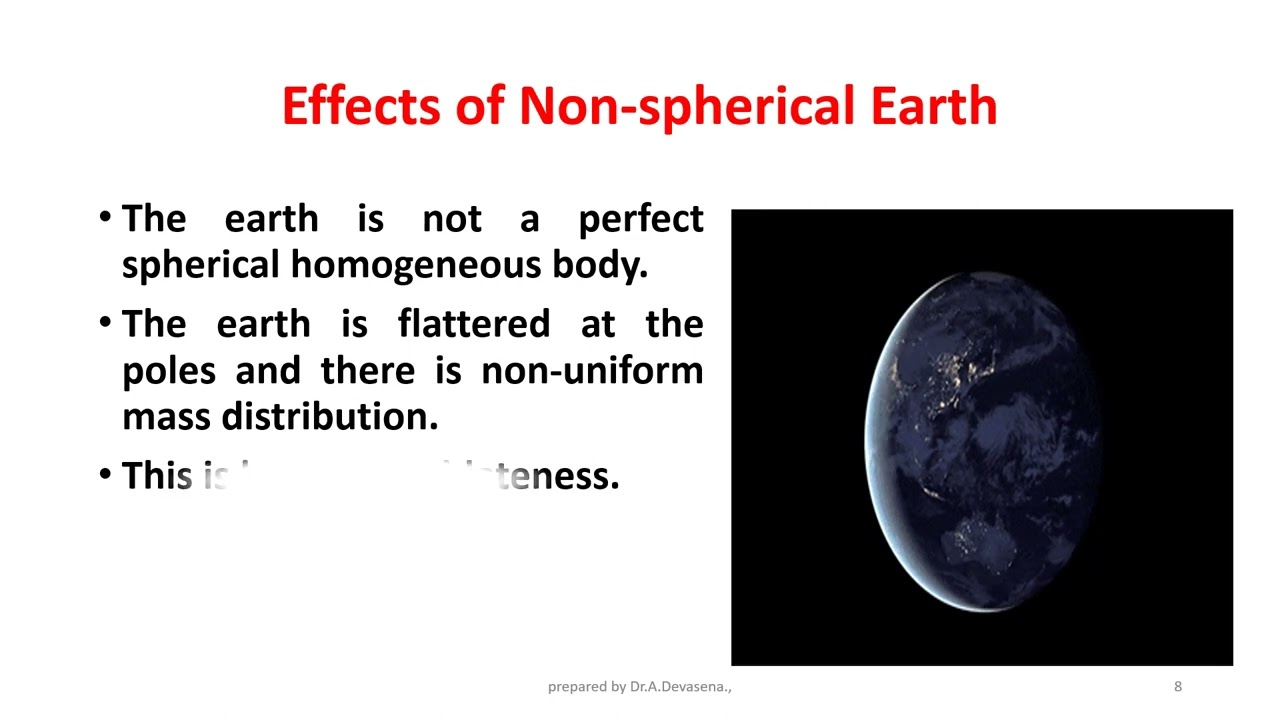
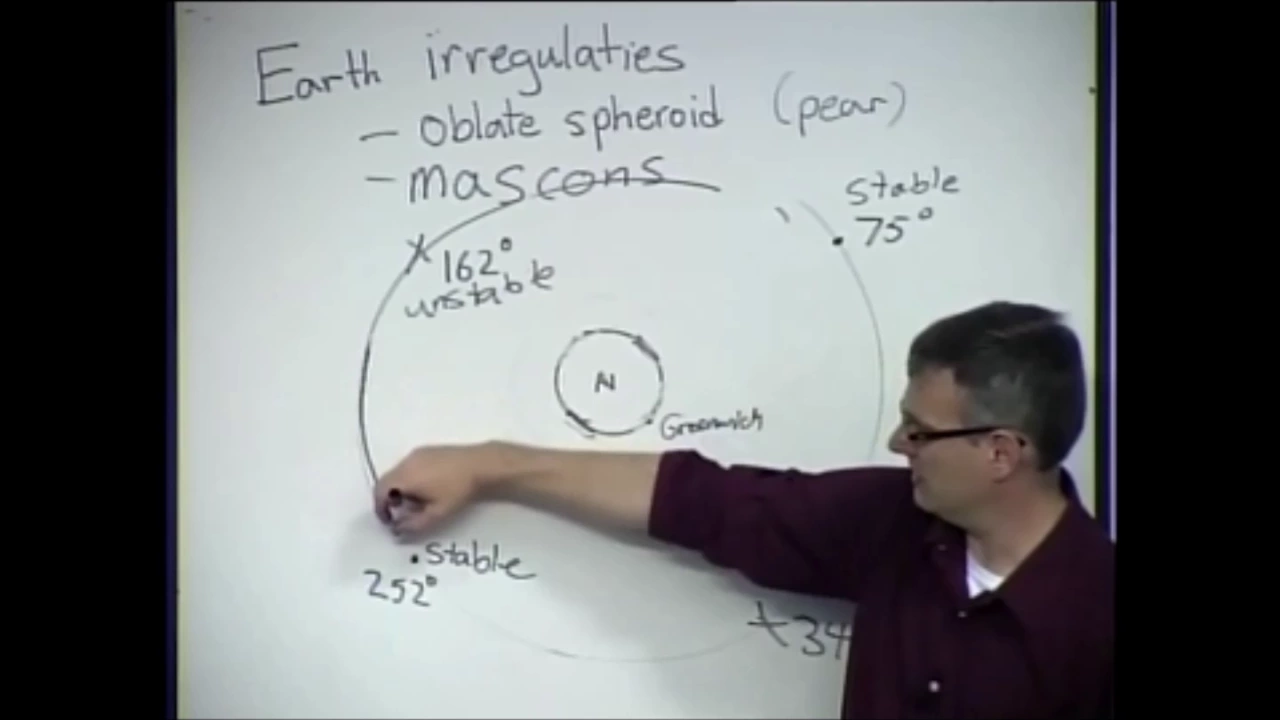
Study of orbital perturbations (such as Earth's J2 oblateness effect, atmospheric drag, and solar radiation pressure) that cause elements to change over time.
Design and analysis of orbital maneuvers, including Hohmann transfers and plane-change maneuvers.
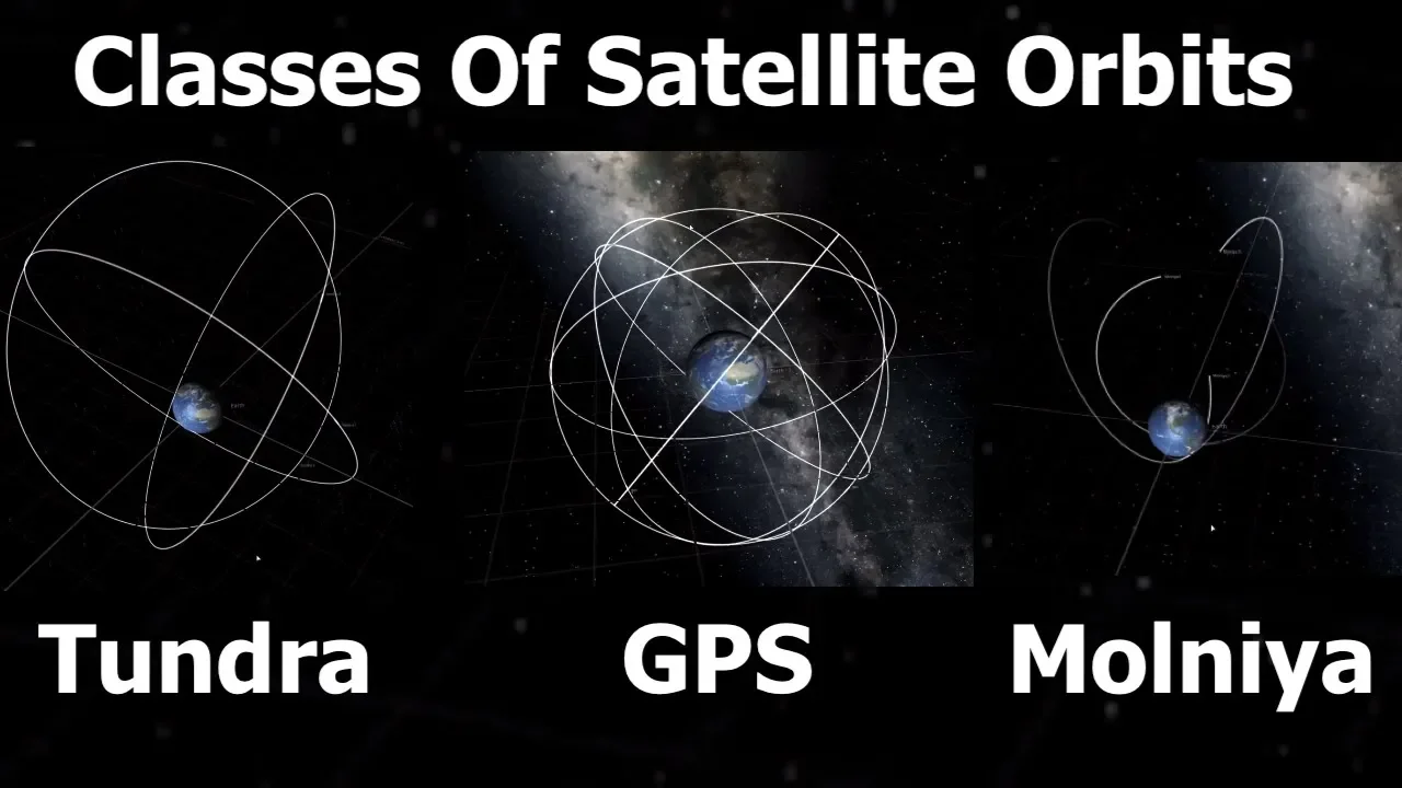
Characteristics of specific real-world orbit types, such as Sun-synchronous, Molniya, and Geostationary orbits.
Orbit determination methodologies, which involve calculating Keplerian elements from raw observational tracking data.
16.8K views330likes9:39Original Release: 2021-12-30
in this video we'll be introducing the kepler and orbital elements which include semi-major axis eccentricity the orientation of the peripheral frame with respect to the inertial frame with the three angles orbital inclination right ascension of the ascending node and argument of periapsis and then finishing with true anomaly and i recommend that you follow along with this video using astronomics interactive demo which can be found at this url which is deployed by github pages and i'll have a link in the description to it and also a link to the video which explains how to use it we'll start with some major axis and eccentricity which correspond to the size and shape of an orbit so here we have earth milky way in the background an elliptical orbit and a spacecraft currently at this position shown by its position vector r so to begin we need to define two points in this orbit where the first is periapsis which is the point closest to the center of the earth in the orbit and the second is apoapsis which is the farthest point the line connecting these two points is called the abs line using just these two scalar values apoapsis and periapsis we can calculate our semi-major axis and eccentricity with a semi-major axis is simply the average of the apoapsis in the periapsis which geometrically corresponds to half of the apps line so that major axis is the only element needed to calculate orbital period so no matter how orbits look if two of them have the same semi-major axis they have the same orbital period and here's the equation calculating eccentricity using these two values and there are a few interesting things to notice about this equation where first the equation must be greater than or equal to zero it cannot be negative because apoapsis is defined to be greater than or equal to periapsis and this equation is equal to zero when apopsis and periapsis are equal to each other which would only be true in a circular orbit where all points are equidistant to the center of the earth which is a definition of a circle however this equation only applies to elliptical orbits in this form which are defined as having an eccentricity between zero and one so the closer it is to zero the more circular the orbit is the closer it is to one the more elliptical the orbit is however we can rearrange that equation to get to this equation which applies to all orbits since for parabolic and hyperbolic orbits the semi-major axis is defined as negative however we're going to focus on elliptical orbits here and go over the other types of orbits later in the series next up are the three orbital elements that describe the orbital plane with respect to the inertial frame so if you're unfamiliar with 3d rotations and euler angles no worries the most important and straightforward angle to understand is the inclination which we'll be going over by itself in the next slide and for those who are familiar with euler angles the right ascension inclination and argument of periapsis are the angles of a 313 euler angle sequence that describes the rotation between the inertial frame and the perifocal frame where the peripheral frame is inertial and defined as the x-axis pointing towards periapsis z-axis pointing in the angular momentum direction which is perpendicular to the orbital plane and y-axis completes the right-handed system and we'll be going deeper into those details later in the series but for now we'll just focus individually on each of the three angles we'll start with the orbital inclination which again for now is the most important and straightforward to visualize orbital inclination is angle between the equatorial plane and the orbital plane so on the right here we have several different examples to visualize inclination in three dimensions where here the red orbit has an inclination of zero degrees meaning that it is always above earth's equator which we can also see in its ground track that is a straight line at latitude equals zero degrees next is a 45 degree inclination orbit where we can clearly see that the angle between the red orbit and the green is 45 degrees and we can also read the inclination of an orbit from a ground track by observing the highest latitude that the orbit reaches so in the ground track the highest latitude the green orbit goes to is 45 degrees therefore it is a 45 degree inclination orbit and same with a 75 degree inclination orbit it has a bit of a different shape but we just need to check for the highest latitude and this also applies to the negative lowest latitude so the lowest latitude this orbit will reach is negative 75 degrees or 75 degrees south overall inclination can also tell us if an orbit is pro grade or retrograde so anywhere between 0 and 90 degrees is a pro-grade orbit 90 degrees is a polar orbit and greater than 90 degrees is retrograde so the purple orbit here with an inclination of 100 degrees is a retrograde orbit and sun synchronous orbits are an application of these types of near polar retrograde orbits and it's also valid to think of retrograde orbits as having a negative value for inclination with a negative sign tells you that it is retrograde and the value tells you the angle between the equatorial plane and the orbital plane so for this 100 degree inclination orbit it's equivalent to say that it's a negative 80 degree inclination orbit and we can again verify that with the ground track to see it the highest latitude this orbit reaches is 80 degrees so here would be a good time to experiment with astrodynamics interactive demo seeing how the inclination changes the 3d plots and the ground tracks so for example here the green orbit is nearly circular and 60 degrees inclination same with red except for zero inclination so again we can see that it stays the zero inclination orbit stays along the earth's equator and the maximum that latitude that the green orbit sees is about 60 degrees up here and negative 60 down here and we can mess around with this and say we want 120 degrees inclination which again would mean that would be negative 60 degrees inclination which means it is retrograde as we can see here in the 3d plot and again we can see at the highest latitude it reaches is again 60 degrees latitude next up is the right ascension of the ascending node sometimes called longitude of the ascending node which is defined as an angle between the inertial x-axis which is the red vector here and the ascending node where the ascending node is a point in the orbit where the spacecraft comes up through the orbital plane over the z component of position crosses from negative to positive the red plot here has zero ran since that point where the orbit comes up through the equatorial plane is right on the x-axis here and the green orbit has a 30 degree rand since that point is 30 degrees from the x-axis so again going to aid we can experiment with the right ascension here where we have again two orbits the green is 60 degrees inclination in a rand of 30 degrees and same with a red except with a rand of zero degrees so for the red we see that it comes up through the equatorial plane right at the x-axis which is this is the x-axis with the red point at the end and then we can see for the green orbit that it's 30 degrees from that where it comes up through the equatorial plane and again we can change these numbers and say we want to go to again 120 propagate those orbits and then we can see now that this is 120 degrees away where the green orbit crosses up through the equatorial plane and i should mention also that when they go back down to the orbital to the equatorial plane which is z component going from positive to negative that's called the descending node last up is argument of periapsis which is defined as the angle between the ascending node and the orbit periapsis this one's a bit harder to visualize so we'll do it with the aid tool but real quick these two orbits have a difference of 180 degrees of argument of periapsis so their periapsis points are on opposite sides of the earth so here we have those two orbits they're a little bit bigger semi-major axis eccentricity of 0.3 inclination of 60 degrees they both have a rand of 30 degrees but the green orbit has an aggregate of periapsis of 180 degrees and we'll see how they differ so first up because they both have a rand of 30 degrees they both cross the equatorial plane right at 30 degrees from the x-axis so we can see that here that they have the same right ascension of the ascending node but the difference here is going to be the argument of periapsis where since for the red orbit is equal to zero that means the ascending node and the periapsis are at the exact same place so periapsis for the red orbit is right there where it crosses up to the equatorial plane but for the green orbit that is 180 degrees later so it's exactly on the opposite side here of the earth and again i encourage you to experiment a lot with this because it's going to be a lot more helpful if you just mess around with the numbers and see how everything changes for example say we change the argument of periapsis so instead of 180 degrees to 90 degrees where would you expect for the periapsis to be and it should be around 90 degrees which should be around the z axis over here so let's go ahead and check that propagate orbits and we can see that the periapsis is again somewhere over here about 90 degrees away from where the red one is and finally the last orbital element is true anomaly which describes the position of the spacecraft along its orbit and is the only element that changes with respect to time in the two-body problem so true anomaly is defined as an angle between a periapsis and its current position so if we take a look in the plot on the left at time equals zero the spacecraft is at periapsis since true anomaly equals zero true anomaly then increases rapidly at first but slows down a spacecraft approaches apoapsis because of the inverse relationship between position and velocity so as position magnitude increases velocity magnitude decreases then true anomaly hits apoapsis at 180 degrees and begins to speed up again since the spacecraft is now on its way back to periapsis and the process repeats and note that there also exists mean anomaly and eccentric anomaly that describe where the spacecraft is a bit differently and we'll be getting to those later in the series as well which come up in kepler's equation that is a transcendental equation because given a mean anomaly you cannot algebraically solve for eccentric anomaly you have to do so either using a root solver method or series expansion in the next video we'll be going over the perifocal reference frame since we will need it to understand it in order to convert back and forth between state vector which is position and velocity and the kepler and orbital elements so let me know if you have any questions or comments about this video be sure to hit like and subscribe if you liked it and share it with any others who you think would find useful and i'll see you in the next one
Up Next

8:50
Nanomaterials Engineering: Applications and Properties
@crashcourse
263.1K views•2018-11-01

30:32
Ultrasonic Transducers: Resonant Frequency Measurement and Horn Design
@imajeenyus42
229.9K views•2017-02-22

54:16
Polymer Environmental Degradation: Mechanisms & Stabilization
@iit
1.8K views•2012-07-10

33:39
How a Student's Question Saved a NYC Skyscraper from Collapse
@veritasium
22.8M views•2025-04-26
Related Study Plans & Knowledge Roadmaps
Structured learning paths in Engineering
engineering
Building Acoustic Levitators: Physics & Arduino
01The Physics of Sound and Standing Waves
02Piezoelectric Transducers and H-Bridge Drivers
03Arduino Programming: Generating 40 kHz Signals
+ 2 more learning modules
14h5 modules
Explore Roadmap
engineering
Building Peltier Cloud Chambers: Particle Tracks
01Cosmic Rays & Cloud Chamber Physics
02Thermoelectric Cooling (TEC) Fundamentals
03Custom Liquid-Cooling Loop Design
+ 2 more learning modules
18h5 modules
Explore Roadmap
engineering
Yagi-Uda Antennas: Modeling, Build & VNA Test
01Introduction to RF and Antenna Fundamentals
02Yagi-Uda Antenna Design Principles
03Antenna Modeling and Simulation in 4NEC2
+ 2 more learning modules
18h5 modules
Explore Roadmap
engineering
ECG Monitor Design: Op-Amps, Filters & Noise
01Electronics & Breadboard Basics
02Op-Amps and Instrumentation Amplifiers
03Bioelectricity and ECG Fundamentals
+ 2 more learning modules
18h5 modules
Explore Roadmap