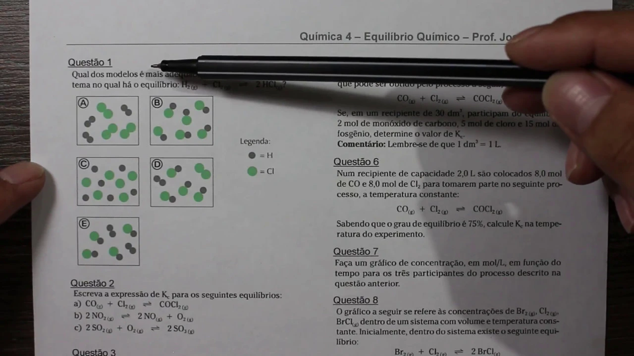


![[FULL] - BÀI 1 - KHÁI NIỆM CÂN BẰNG HÓA HỌC (CHƯƠNG TRÌNH MỚI)](https://i.ytimg.com/vi_webp/BZYzJPbJ1nc/maxresdefault.webp)


![[Hóa 11] Cân Bằng Trong Dung Dịch Nước (Sách Chân Trời Sáng Tạo, Kết Nối Tri Thức Với Cuộc Sống)](https://i.ytimg.com/vi/eVvlVnGQ3IU/sddefault.jpg)

























The solubility product constant (Ksp) is an equilibrium constant that quantifies the extent to which an ionic compound dissolves in water, representing the product of the concentrations of its dissolved ions each raised to the power of their stoichiometric coefficients; compounds with smaller Ksp values are less soluble, and Ksp can be used to calculate either the solubility of a compound from its Ksp value or to determine the Ksp value from measured ion concentrations in a saturated solution.
Understand the Solubility Product Constant Ksp in Chemistry
Added:Understanding of dynamic chemical equilibrium and how to write basic equilibrium constant (Kc) expressions.
Ability to write balanced dissociation equations for ionic compounds dissolving in aqueous solutions.
Fundamental concepts of solution chemistry, specifically molarity (mol/L) and chemical stoichiometry.
Prior exposure to the basic structure of ICE (Initial, Change, Equilibrium) tables used in general equilibrium problems.
The Common Ion Effect and how the addition of a shared ion reduces the molar solubility of a salt.
Predicting precipitation by comparing the ion product / reaction quotient (Qsp) to the solubility product constant (Ksp).
Analyzing the impact of pH on solubility, particularly for salts containing basic anions like carbonates or hydroxides.
Selective precipitation, which involves separating different metal ions in a solution based on their differing Ksp values.
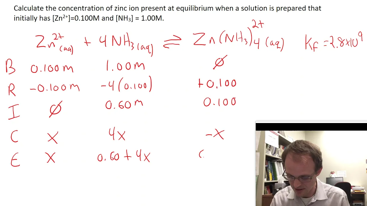
Complex ion formation (Kf) and its role in increasing the solubility of otherwise insoluble precipitates.
460.9K views8.9Klikes8:36Original Release: 2019-05-31
Professor Dave here, let’s talk solubility.
When we first discussed solubility, we learned that some ionic compounds are water soluble, and will completely disperse in solution, due to the ion-dipole interactions they will make with water molecules.
We also learned that other ionic compounds are water insoluble, and will not dissolve at all, remaining completely in the solid phase.
Beyond this, if the components of such a compound find each other in solution, they will precipitate, and leave solution completely to form a solid.
This is actually a slight oversimplification that served its purpose at the moment, but now it’s time to get a more sophisticated and quantitative understanding of solubility, so let’s get a closer look.
It’s true that many ionic compounds are completely soluble, but the reality is that even the ones that we call insoluble will dissolve to a minuscule degree.
Whatever the degree to which dissolution occurs for a particular substance, we can communicate this using the solubility product, abbreviated as Ksp.
Let’s look at a substance like silver chloride, which we label as water insoluble.
As we said, if there is an excess of it in water, it will dissolve to a tiny extent and cause a dynamic equilibrium.
Some ions dissolve as other ions rejoin the lattice.
Just as with any other type of equilibrium, there must be an equilibrium constant to describe it, and that’s the solubility product.
As we might guess, this will simply be equal to the product of the two ion concentrations in solution, each raised to the power of their stoichiometric coefficients, which in this case is simply one and one.
Notice that we do not include the solid itself in this expression, as we do not include solids in equilibrium expressions.
The smaller the constant, the fewer the ions that will be present in solution, and therefore the less soluble the substance must be.
And compounds that are extremely water insoluble will have Ksp values on the order of ten to the negative thirty, negative fifty, or even smaller.
Let’s make sure we can write these solubility products for various equilibria.
Take something like calcium carbonate.
First, we must write out the complete equilibrium.
Upon dissociating, this will form a calcium ion and a carbonate ion.
Therefore, the solubility product will be equal to the product of these two ion concentrations.
If we have something like magnesium hydroxide, it’s the same thing, except that dissociation produces one magnesium ion and two hydroxide ions, which means that hydroxide ion concentration will be squared in the solubility product expression.
We can even do this for something more complicated, like apatite, which is a mineral.
This will dissociate into five calcium ions, three phosphate ions, and a hydroxide ion, so the solubility product expression will look like this.
In this way, a number of ionic compounds that we previously deemed insoluble should actually be categorized as slightly soluble.
If we have a way of measuring ion concentrations in solution, we can calculate the Ksp value for a given substance.
Let’s say we have a saturated solution of milk of magnesia, which is magnesium hydroxide.
This is slightly soluble and dissolves according to the following equilibrium.
Say we measure the resulting magnesium ion concentration as being 3.7 x 10^-6 molar.
What will be the solubility product for magnesium hydroxide?
First let’s write the Ksp expression for this substance, which we derived earlier.
Notice that hydroxide concentration is squared due to the coefficient in the equilibrium.
Now if this is the concentration of the magnesium ion, then the hydroxide ion concentration must be precisely double, since there are two hydroxide ions for every magnesium ion in this substance.
So all we need to do is plug these two concentrations into the expression, evaluate, and we will get 2.0 x 10^-13 for Ksp, which will be a unitless constant, just like other equilibrium constants.
We can also go the other way around, and predict the concentrations of ions that will result in solution when dissolving a substance with a given Ksp.
Let’s say we place copper one bromide, which has a Ksp of 6.3 x 10^-9, in aqueous solution, which will then generate copper ions and bromide ions to some extent.
What will be the molar solubility of this substance, meaning how many moles per liter of the formula unit will dissolve?
To find this, we can write the solubility product expression, and use this to construct a simple ICE chart.
In this, we will not list any values for copper bromide, as this is a solid.
The ions themselves will start at zero, the change will be X because of the 1 to 1 to 1 ratio, and this means that the equilibrium concentrations of the ions will also be equal to X. Therefore the Ksp will be equal to X^2, and X will be 7.9 x 10^-5 moles per liter.
This is the molar solubility of copper one bromide, which in this case is simply the concentration of copper ions and bromide ions in solution at equilibrium.
This can be a little trickier if the Ksp equation involves exponents, but the process is essentially the same.
Let’s look at calcium hydroxide, which has a Ksp of 8.0 x 10^-6.
Say we place this in aqueous solution, which will produce some calcium ions and hydroxide ions.
Again, let’s write the Ksp expression, noticing that the hydroxide concentration must be squared, as there will be two hydroxide ions for every formula unit of calcium hydroxide that dissolves.
Then when we make the ICE chart, we will notice that again the initial concentration of each ion will be zero, but the change will be X and 2X respectively, due to the stoichiometry of the equation, and the equilibrium concentrations will also be X and 2X.
Putting these into the Ksp expression, we get that the Ksp will be equal to 4X^3.
Now solving for X, we divide by four and then take the cube root, leaving us with 1.3 x 10^-2 for X, which will therefore be the molar solubility, which we can interpret as the solubility of the solid expressed in moles per liter, or the moles of the solid that will dissolve per liter of water.
So now that we’ve learned a bit about the solubility product, it’s time to learn a few applications of this concept.
But first, let’s check comprehension.
Up Next

97:40
Extreme Acid Mine Drainage at Iron Mountain, California | USGS Lecture
@USGSPresentations
2.7K views•2018-08-09
24:04
The Jablonski Diagram: Radiative and Non-Radiative Transitions | Photochemistry
@benedictugi8420
262 views•2025-07-15
10:45
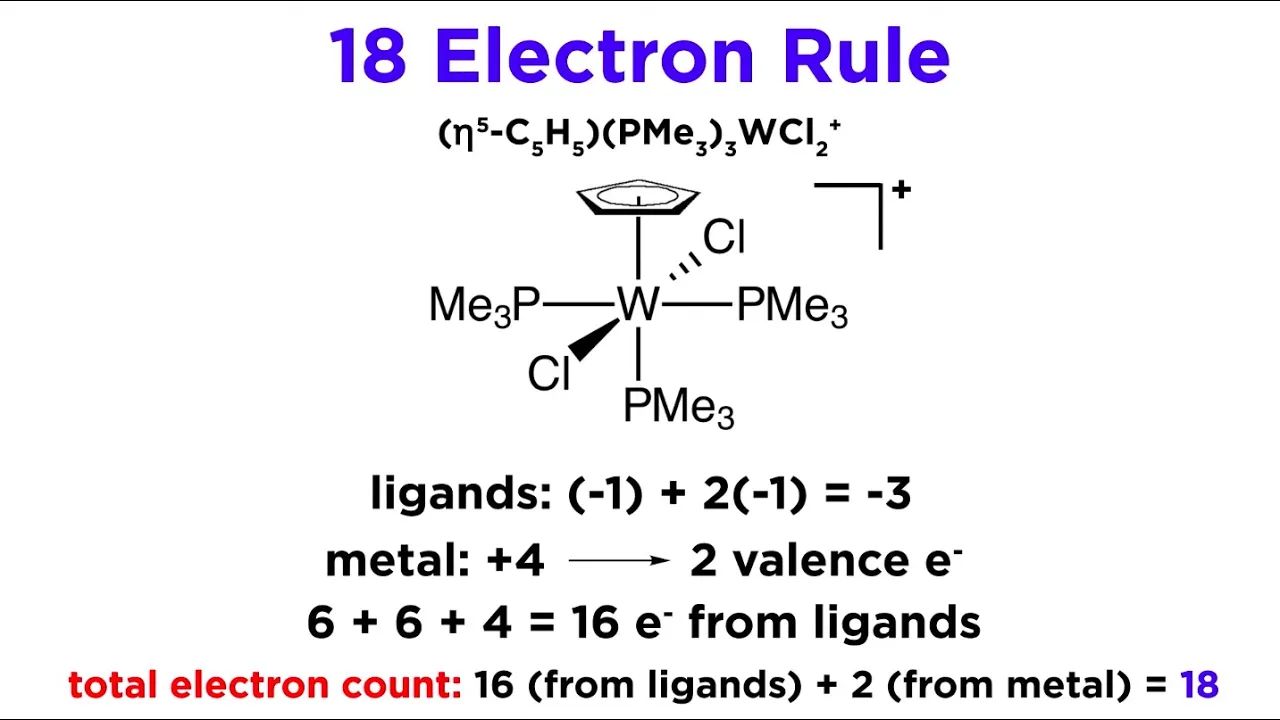
18 Electron Rule in Transition Metal Complexes | Stability & Electron Counting
@ProfessorDaveExplains
176.2K views•2022-09-28

17:31
Edible Water Bottles: A DIY Guide to Sodium Alginate Spherification
@ryan
10.5M views•2019-06-21
Related Study Plans & Knowledge Roadmaps
Structured learning paths in Chemistry
chemistry
Photochemistry: Excited States & Reactions
01Foundations of Light-Matter Interactions
02Molecular Orbitals and Electronic States
03Photophysical Processes and Jablonski Diagrams
+ 2 more learning modules
18h5 modules
Explore Roadmap
chemistry
Coordination Chemistry: Bonding & Properties
01Introduction to Transition Metals and Ligands
02Crystal Field Theory (CFT) and Geometry
03Magnetic Behavior and Spin States
+ 2 more learning modules
14h5 modules
Explore Roadmap
chemistry
Polymer Chemistry: Synthesis & Properties
01Introduction to Macromolecules & Monomers
02Polymerization Synthesis Mechanisms
03Polymer Characterization Techniques
+ 2 more learning modules
12h5 modules
Explore Roadmap
chemistry
Separation Science: GC, HPLC & Mass Spec
01Foundations of Separation Science
02Gas Chromatography (GC) Principles & Systems
03High-Performance Liquid Chromatography (HPLC)
+ 2 more learning modules
24h5 modules
Explore Roadmap