












![1. Introduction [Theoretical Physics (Path Integral) SC514231 KKU 2021]](https://i.ytimg.com/vi/NZa3kMq0jYM/hqdefault.jpg)
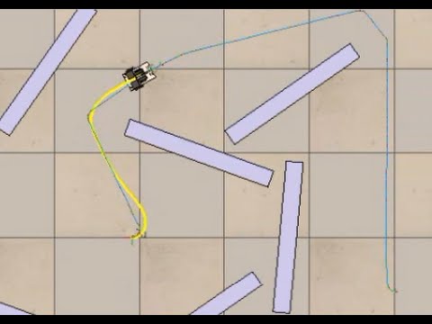









This tutorial derives the kinematics equations for differential drive robots, showing how the robot's linear velocity (x_dot, y_dot) and angular velocity (theta_dot) can be predicted from the angular velocities of the left and right wheels using the equations: x_dot = (R/2)(ω_L + ω_R)cos(θ) - (R/s)(ω_L - ω_R)sin(θ), y_dot = (R/2)(ω_L + ω_R)sin(θ) + (R/s)(ω_L - ω_R)cos(θ), and theta_dot = (R/s)(ω_L - ω_R), where R is the wheel radius, s is the distance between wheel centers, and ω_L and ω_R are the angular velocities of the left and right wheels respectively.
Deriving Differential Drive Robot Kinematics: Equations Explained
Added:Basic rigid body 2D kinematics, including the relationship between linear velocity, angular velocity, and radius of rotation.
Fundamentals of coordinate frames, vector translation, and basic trigonometry (sine and cosine).
Introductory differential calculus, specifically understanding rates of change and derivatives with respect to time.
The concept of the 'pure rolling' (no-slip) constraint for wheels on a surface.
Deriving and solving the Inverse Kinematics equations to calculate wheel velocities from desired robot trajectories.
Implementing Odometry and Dead Reckoning algorithms to estimate a robot's position and orientation over time using wheel encoder data.
Designing closed-loop motion controllers, such as PID or Pure Pursuit, for trajectory tracking of differential drive robots.
Transitioning from kinematics to dynamics, exploring how forces, torques, mass, and inertia affect robot motion.
22.7K views757likes16:27Original Release: 2023-10-28
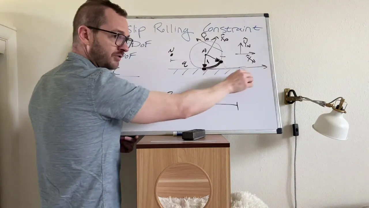
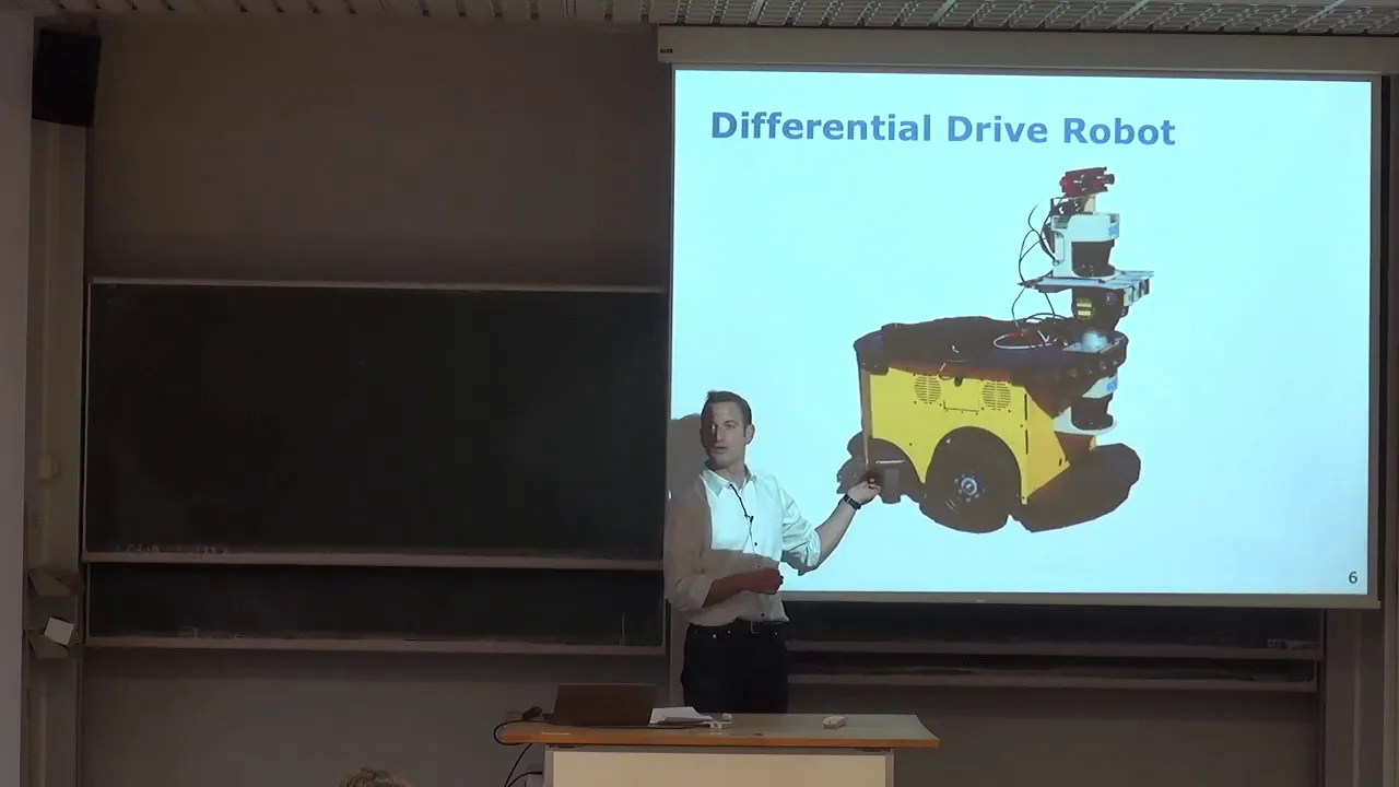
hello everyone and welcome to mechatronics and Robotics tutorials in this tutorial we provide clear and detailed explanation of kinematics equations and geometry of motion of differential build robot or differential Drive robot in the first part of this tutorial that you're are currently watching we will derive the equations describing the kinematics of the differential Drive robot in the second part of the tutorial we will explain how to solve the forward kinematics problem and how to simulate the robot in Python and in the third part of this tutorial we will explain how to solve the inverse kinematics problem but before I start with explanations and derivations I would like to mention the following it took me a significant amount of time energy in planning to create this completely free video tutorial as well as more than 300 50 free video tutorials that you can find on my YouTube channel and consequently I kindly ask you to press the like And subscribe buttons thanks a lot over here you can see an example of a differential Drive robot here's the photograph of the differential Drive robot the robot consists of two wheels wheel one and wheel 2 that are driven by two DC motors over here here is the first DC motor the robot body is supported by Caster wheel here's the Caster wheel it's a passive wheel and it's not being actively moved this figure shows the top view of the differential Drive robot after a few geometrical simplifications that do not affect the model generality we have two wheels left wheel and right wheel and here's the robot base we can observe three velocities VL VB and VR the point L is the center of the left wheel the point R is the center of the right wheel and the point B is the point on the line connecting L and R and this point sits at the middle of this line the velocity VL is the velocity of the center point of the left wheel similarly the velocity VR is the velocity of the center point of the right wheel these velocities are a direct consequence of the fact that the wheels are spinning due to the Torx exerted by the motors in this figure the robot is turning left this is because the intensity of the Velocity VR is larger than the intensity of the Velocity VL in fact as we will explain later in this configuration all the three points l b and R will describe concentric circles centered at the instantaneous Center of rotation this point is also known as the instant Center of rotation or the instantaneous velocity Center here it's very important to emphasize the following we can completely control the robot's motion by controlling the right and left wheel angular velocities or the right and left wheel rotational angles the velocities VL and VR are linearly proportional to the angular velocities of the right and left Wheels next let us illustrate several motion scenarios in this scenario the robot is moving straight this is because the intensities of the velocities VL and VR are equal consequently in the instantaneous Center of rotation is at infinity and all the points describe straight lines that is this point describes the straight line this point describes the straight line and this point describes the straight line in this scenario the robot is moving right this is because the intensity of the Velocity VL is larger than the intensity of the Velocity VR and consequently the robot will turn right next let us look at this scenario over here the robot is rotating around the point B in this case the intensity of the Velocity VL is equal to int it of the Velocity VR however these two velocities have opposite directions and consequently the robot will spin in the clockwise direction to conclude by changing the velocities of the centers of the wheels or equivalently by changing the angular velocities of two wheels we can control the robot's motion we can either turn left right or spin around or even go along the straight line in the SQL we provide a detailed kinematic analysis of the differential Drive robot we want to establish the equations that will relate the angular velocities of the two wheels with the velocity of the center of the robot and the angular velocity of robot's rotation let's Analyze This figure the coordinate system X Y is a fixed or inertial coordinate system on the other hand the coordinate system XB YB is located at the center B this coordinate system is rigidly attached to the robot's body and often it's called the body coordinate system or the body frame of the robot the point C is the instantaneous Center of rotation from the velocity analysis perspective during a short time interval the robot seems to rotate around the instantaneous Center of rotation this point is constructed by finding an intersection of the line connecting the top of the Velocity Arrows with the line passing through the centers of the wheels that is we basically construct the line starting from here then going to this point and we just draw a straight line and then we find intersection with this line the line that passes through b and has this direction it's perpendicular to XB and this will Define the instantaneous Center of rotation the symbol Omega denotes the instantaneous angular velocity this angle Theta is the rotation angle of the robot's body this angle is at the same time the rotation of the body frame with respect to the inertial frame XY under the assumption that the intensities of the velocities are not changing during the time interval the points l b and R describe a circular trajectories centered at the point C and this is Illustrated in this figure over here you can see a detailed kinematic diagram of the robot and let's explain all the symbols and quantities such that you can understand the ations X and Y are the translation coordinates of the body frame attached to the point B with respect to the inertial frame X and Y Theta is the angle of rotation of the robot which is at the same time the angle between the body frame and the inertial frame XB and YB are the coordinates in the body frame and at the same time they denote the access of of the body frame XB and YB C is the instantaneous Center of rotation Omega is the instantaneous angular velocity of the robot body L is the center point of the left wheel R is the center point of the right wheel B that is the point over here is the middle point between the points L and R VL is the velocity of the center of the left wheel VR is the velocity of the center of the right wheel VB is the velocity of the point b f l is the angular velocity of the left wheel fi R is the angular velocity of the right wheel L is the distance between the point B and the point C that is the point of instantaneous Center rotation R is the radius of the wheels s is the distance between the points lnr x dot is the projection of the Velocity VB with respect to the x axis and y dot is the projection of the Velocity VB onto the Y AIS in the SQL we will derive the equations that relate F and F with x dot y Dot and Tera dot these equations will enable us to predict the robot Center Point velocity as well as the angular velocity as the functions of the control variables f l and f r that is we start from the assumption that the following quantities and parameters are known file f s r and we want to determine Tera dot x dot and Y dot let's derive the equations over here you can see this very important kin itic diagram and focus over here if you don't know any quantity or if you need an explanation just look over here let's start from this figure and first let's Express VL and VR as functions of Omega and L obviously from this graph we have that v l is Omega time this distance from L to C and this distance is nothing less than lus Us s/ 2 where s is this distance similarly we obtain that VR is Omega times this distance from here to here and this distance is L + s/ two and consequently we obtain these two equations now the issue with these two equations is that both L and Omega are not known consequently we need to solve these two equations for L and Omega starting from this first equation we can express Omega like this then by substituting this equation in this equation and by manipulating the resulting equation we can finally obtain the expression for L Now by substituting this equation in the first equation that is in the expression for VL we finally obtain this expression and by manipulating this expression we can find the expression for Omega so Omega is simply v r minus VL / s divided by this distance and this is very important now for clarity let us repeat these two expressions that is the expression for L and expression for Omega and these two equations are very important for our next derivation next let's analyze figure eight what is x dot let's see x dot is the projection of VB on the x inertial axis and that's obviously VB cosinus this angle Theta similarly y dot is VB sinus Theta and Theta dot is nothing less than Omega this is a very important observation and this follows from the fact that the angles are perpendicular to each other or better to say they're equal for example you have this angle and you have this angle obviously these angles are equal mainly because they have perpendicular sides this side is perpendicular to this side and this side is perpendicular to this side consequently this will be angle Theta and Omega is nothing less than the first derivative of theta and that's the last equation over here let's continue these three equations can be written like this in a compact Vector Matrix form on the other hand we have that the intensity of the Velocity VB is equal to Omega * L * the distance now by substituting L on Omega in this equation we obtain this equation that is this form VB is simply VR + VL / 2 Now by combining this equation with the equation for Omega that is with this equation we finally obtain the equations given in 12 these two equations can be written like this what's the importance of these equations these equations enable us to predict VB and omega as functions of VL and VR and keep in mind that we can control VL and VR since we can control the spinning of motors Now by substituting this equation that is the equation 13 into the equation 9 we obtain this equation and after multiplying this part or better to say this Matrix with this Matrix we obtain this equation and this system of equations can be expanded and finally we obtain the system the system of equations 15 relates the controlled wield velocities VR and VL with the velocity projections of the center B of the robot and the angular velocity of the robot it's a very important kinematic equation however we know that the ve velocities are actually functions of the ve angular velocities f l dot and f r dot let's observe this figure since the radius is R we can say that VL is R * f l dot similarly VR is equal to R * f r dot these two equations can be written compactly like this by substituting this equation in equation 14 over here we obtain the equation 18 here's the first equation and once we multiply this matrix by this Matrix we obtain the final form this last equation can be written in the expanded form that is we obtain the expression for x dot expression for y Dot and expression for Tera Dot and this equation is the final derived equation in this tutorial it relates the angular velocities of the left and right Wheels with x dot y Dot and Tera dot that is this equation enables us to predict the global robot velocities and angular velocity as functions as Lo of local joint velocities and this is very important also this equation will enable us to predict the robot trajectory and to solve the direct and inverse kinematic problems okay that would be all for today I hope that you like this video if you like the videos I'm creating please press the like And subscribe buttons thanks a lot and have a nice day
Up Next

42:15
Wheeled Robot Control: Differential Drive Odometry Tutorial
@ccirobotics8123
53.2K views•2019-09-11

58:25
MathWorks Virtual RoboSub Simulation Environment | Webinar 2026
@RoboNationInc
209 views•2026-03-10

11:04
How to Build a Self-Balancing Robot: Arduino Nano & MPU6050
@easytechzones
16.8K views•2022-03-09

25:22
Micromouse: The Fastest Maze-Solving Robots on Earth
@veritasium
23.5M views•2023-05-24
Related Study Plans & Knowledge Roadmaps
Structured learning paths in Robotics
robotics
Building Delta Robots: Kinematics & Pico
01Foundations of Delta Robots & Mechanical Design
02Electronics and Microcontroller Setup with Pi Pico
03Delta Robot Kinematics and Coordinate Math
+ 3 more learning modules
65h6 modules
Explore Roadmap
robotics
Building Ballbots: Dynamics, Kalman & LQR
01Embedded Electronics & Omniwheel Actuation
02Ballbot Kinematics & Rigid Body Dynamics
03IMU Sensors & Kalman Filter State Estimation
+ 2 more learning modules
42h5 modules
Explore Roadmap
robotics
Micromouse: Hardware, PID Control & Flood-Fill
01Electronics & Teensy Microcontroller Basics
02Sensors and Actuators: Motors, Encoders & IR
03Precision Movement: Implementing PID Control
+ 2 more learning modules
35h5 modules
Explore Roadmap
robotics
CDPR: Kinematics, Arduino & Winch Control
01Foundations of Arduino & Basic Electronics
02Stepper Motors and Winch Mechanics
03Kinematics of 2D Cable-Driven Robots
+ 2 more learning modules
28h5 modules
Explore Roadmap