Stepper motors offer simpler open-loop operation with lower cost and faster startup (200-400ms) but have limited accuracy (up to 25,600 steps/rev) and cannot handle overload, while servo motors provide superior accuracy (131,072 PES with 17-bit encoders), closed-loop feedback, and overload capability at higher cost and complexity; stepper motors suit applications requiring simple operation, minimal positional errors, and budget constraints, whereas servo motors excel in precision positioning and variable load scenarios.
Stepper vs Servo Motors: Accuracy, Control & Cost Guide
Added:Deep Dive
Basic principles of electromagnetism and how electric motors generate torque.
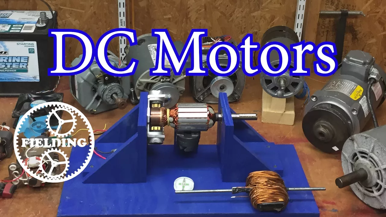
How Motors Work For Beginners (Episode 1): The DC Motor: 032
2.6M
This segment covers three foundational electromagnetic principles. First, magnets with like poles repel each other when facing each other. Second, electromagnetic induction requires three elements: a magnetic field source, a conductor, and relative motion between them—demonstrated by generating voltage when a magnet passes a wire. Third, current-carrying wires produce magnetic fields strong enough to visibly affect other magnets. These principles form the basis for understanding how motors convert electrical energy into mechanical motion.
Click to watch →

How is Torque produced in Motor ? | Mayank Sahu
506
This comprehensive section explains how torque is generated in motors through electromagnetic principles. The right-hand thumb rule determines magnetic field direction around current-carrying conductors. Motors consist of a stator (stationary part with main magnetic field windings) and rotor (rotating part with armature conductors). Current direction is represented using dot and cross notation. When current flows through rotor conductors placed in the stator's magnetic field, electromagnetic forces are generated. A single conductor cannot produce torque because forces would act in the same direction. Motors use coils with conductors on opposite rotor sides, creating forces in opposite directions. The flux path distortion creates forces that generate electromagnetic torque (interaction torque), causing rotation. Fleming's Left-Hand Rule (thumb for force, index finger for magnetic field, middle finger for current) determines force direction. Understanding these fundamental principles is essential for mastering electrical machines.
Click to watch →

Warum dreht sich ein Elektromotor WIRKLICH Was hinter jeder Bewegung steckt Feynman erklärt
253
Electric current and magnetism are unified phenomena, not separate forces. Hans Christian Oersted discovered in 1820 that current-carrying wires deflect compass needles, proving electricity produces magnetism. Michael Faraday later showed changing magnetic fields induce electric current. James Clerk Maxwell synthesized these discoveries into four equations, revealing electricity and magnetism as aspects of a single electromagnetic field. When current flows through a conductor in a magnetic field, the Lorentz force pushes the conductor perpendicular to both current and field directions. This fundamental principle underlies all electric motors.
Click to watch →

MAGNETIC EFFECT OF CURRENT & EMI 02 - Electromagnet, Motor, Lorentz force | NSEJS Physics
4.1K
An electric motor converts electrical energy into mechanical energy. When a current-carrying coil is placed in a magnetic field, it experiences a torque that causes rotation. The torque is produced because forces act on opposite sides of the coil in opposite directions. This creates a couple that rotates the coil. The instructor explains that motors are used in appliances like washing machines, refrigerators, and mixers.
Click to watch →

المحاضرة الأخيرة الفصل الثالث الدرس الرابع المحرك الكهربى الموتور فيزياء 3ث 2026
348
Electric motors convert electrical energy into mechanical energy, opposite to dynamos. The fundamental principle is torque (عزم الازدواج): when a rectangular coil carries current in a magnetic field, it experiences two equal and opposite forces not on the same line, creating rotational motion. This principle applies to all electric motors including fans, washing machines, and refrigerators.
Click to watch →
Deep Dive
The conceptual difference between open-loop and closed-loop control systems.

Lec-2 Difference between Open loop and closed loop Control System | Control System|R K Classes|Hindi
27.1K
Open loop and closed loop control systems differ fundamentally in behavior, feedback mechanisms, and sensitivity. Open loop systems maintain consistent behavior without feedback, making them simple and economical but highly sensitive to external disturbances. Closed loop systems incorporate feedback paths with sensors/transducers, enabling adaptive behavior and superior disturbance rejection. While open loop systems are inherently stable, closed loop systems can be either stable or unstable depending on feedback type (negative feedback enhances stability, positive feedback may cause instability). The choice between them depends on application requirements for complexity, cost, and performance.
Click to watch →

Control System |State AE/JE 2021 Crash Course | free online Coaching |RSEB AE/JE Crash Course |L- 1
54.8K
Control systems are classified as open loop or closed loop based on feedback mechanism. Open loop systems lack feedback, making them less accurate, more sensitive to disturbances, and unable to reduce errors automatically. Closed loop systems use feedback to compare output with input, enabling automatic error correction, improved stability, and better disturbance rejection. Key differences include: open loop systems are more stable but less accurate, while closed loop systems are more complex but provide superior performance. The choice between them depends on application requirements for accuracy, stability, and disturbance rejection.
Click to watch →
CONTROL SYSTEM - 1 OPEN LOOP & CLOSED LOOP SYSTEM - TAMIL
61.1K
Open-loop systems apply input without feedback, while closed-loop systems use feedback to compare actual output with desired output. Open-loop systems have a simple input-to-output structure with no feedback path. Closed-loop systems include a feedback mechanism that continuously monitors output and adjusts control actions to minimize error. The key difference is that closed-loop systems can compensate for disturbances and maintain desired output despite external variations, making them more suitable for applications requiring precise control.
Click to watch →
![LAZO ABIERTO y LAZO CERRADO ✅ [Sistemas de CONTROL] #009](https://i.ytimg.com/vi_webp/CxGFoeJ7SD8/maxresdefault.webp)
LAZO ABIERTO y LAZO CERRADO ✅ [Sistemas de CONTROL] #009
161.7K
In control systems, an open-loop system controls a process based on pre-programmed instructions without using feedback from the output, making it simple and inexpensive but unable to compensate for disturbances or variations; conversely, a closed-loop (feedback) system continuously monitors the output using sensors, compares it against a desired setpoint, and automatically adjusts the control action to maintain the desired value, providing better performance and disturbance rejection but requiring careful controller tuning to prevent oscillations and instability.
Click to watch →

Stability of Closed Loop Control Systems
271.5K
Open-loop control systems do not use feedback to determine if the system has met its desired state; they don't observe or sense the output. In contrast, closed-loop systems use feedback of the output state to alter the input. The key difference depends on what you label as the reference signal and what is the output. A system can be considered open-loop if the reference doesn't depend on the output of the plant.
Click to watch →
Deep Dive
Fundamentals of rotational mechanics, including angular velocity, torque, and inertia.

JEE: Rotational Motion L6 | Rotational Dynamics | Class 11 | Unacademy JEE | JEE Physics | Namo Kaul
99.7K
Rotational dynamics studies how forces cause rotational motion. The moment of inertia (I) is the rotational equivalent of mass, depending on mass distribution relative to the axis. Torque (τ) causes angular acceleration (α) according to τ = Iα. Angular momentum (L = Iω) is conserved when no external torque acts. For rigid bodies, L = Iω, with direction along the rotation axis (right-hand rule). Angular velocity (ω) is rate of angular position change; angular acceleration (α) is rate of ω change. Kinematic equations: ω = ω₀ + αt, θ = θ₀ + ω₀t + ½αt², ω² = ω₀² + 2α(θ - θ₀).
Click to watch →

Rotational Motion | Part-2 | Mind Maps Series | Physics | NEET 2025 Hindi Medium | Nitin Sir
2.6K
Angular velocity is calculated as ω = v/r, where v is linear velocity and r is distance from the axis. For relative angular velocity between two points, find the relative velocity perpendicular to the line joining them, then divide by the distance. Moment of inertia for a point mass is I = mr², where r is distance from the axis. For systems of point masses, sum individual moments. For two masses m₁ and m₂ separated by distance d, the moment of inertia about the center of mass is I = (m₁m₂/(m₁+m₂))d². For a thin rod of mass m and length l about its center perpendicular to length, I = ml²/12. For a rod about its end, I = ml²/3. For composite systems, sum individual moments and apply parallel axis theorem I = I_cm + md². For a disk, I = mr²/2 about perpendicular axis through center, and I = mr²/4 about diameter. Angular momentum L = Iω, where I is moment of inertia and ω is angular velocity. Convert RPM to rad/s by multiplying by 2π/60. Torque τ = r × F, the cross product of position and force vectors. Magnitude is τ = rF sinθ.
Click to watch →

기초물리 6-1(회전운동과 각운동량)
9K
This comprehensive section covers the foundational concepts of rotational motion. Angular velocity (ω) is defined as the rate of change of angular position, with relationships v = rω and ω = 2π/T. Angular momentum (L) is the rotational equivalent of linear momentum, calculated as L = r × p, with magnitude L = mvr sin(φ). Moment of inertia (I) represents rotational mass, calculated as I = Σmr² for discrete particles or I = ∫r²dm for continuous bodies. Different shapes have different moments of inertia: point mass I = mr², rod about end I = (1/3)mL², rod about center I = (1/12)mL², disk I = (1/2)mr², sphere I = (2/5)mr². The direction of angular velocity and angular momentum follows the right-hand rule.
Click to watch →

L6 : Tourqe and Angular Momentum (Rotation) | Tricks | Physics NEET | Piyush Kamal
293
This comprehensive segment covers the complete fundamentals of rotational mechanics. The instructor explains torque as the rotational equivalent of force, calculated as τ = rF sin(θ), with maximum torque occurring when force is perpendicular to the lever arm. The segment covers angular velocity (ω), angular acceleration (α), and their relationships through equations like ω = ω₀ + αt and τ = Iα. The instructor demonstrates converting angular velocity from rpm to rad/s and solving torque equilibrium problems. The segment also covers angular momentum (L = Iω) and its conservation principle, which states that angular momentum remains constant when no external torque acts on a system. The instructor emphasizes that moment of inertia cannot be zero for any physical body and demonstrates solving problems by equating initial and final angular momentum. The segment concludes with the importance of comprehensive topic coverage for exam preparation.
Click to watch →

حل اسئلة مراجعة الوحدة الثانية _ الحركة الدورانية _ أ.يوسف عودة
306
This comprehensive section covers the foundational principles of rotational motion. Angular momentum is measured in kg·m²/s, while moment of inertia (I = mr²) is measured in kg·m². Angular acceleration (α) is calculated as the change in angular velocity divided by time (α = Δω/Δt). The direction of angular acceleration depends on whether angular velocity is increasing or decreasing—same direction means acceleration, opposite direction means deceleration. Torque (τ) is the rotational equivalent of force, calculated as τ = F × d, where d is the perpendicular distance from the axis of rotation. The general torque formula is τ = r × F × sin(θ), where r is the distance from the axis, F is the force, and θ is the angle between the position vector and force. For irregular objects, the center of mass is closer to the larger mass portion. The center of mass can be found by suspending an object from two different points and finding the intersection of the plumb lines. For equilibrium, the sum of torques about the pivot must be zero (Στ = 0). Moment of inertia depends on mass distribution relative to the axis of rotation—mass farther from the axis increases I. The rotational equivalent of Newton's second law is Στ = Iα, where α is angular acceleration. The relationship between I and α is inverse: larger I means smaller α for constant torque. The rotational kinetic energy is K = (1/2)Iω². For a system with two masses on a rod, the total moment of inertia is the sum of individual moments of inertia: I = Σm_i × r_i². When a rotating body brings mass closer to the axis (like a diver tucking), I decreases and ω increases to conserve angular momentum (L = Iω). For a disk, I = (1/2)mr². The ease of rotation depends on I—smaller I means easier rotation. When the axis passes through the object, I is smaller, making rotation easier.
Click to watch →
Deep Dive
How microcontrollers or PLCs send digital pulses to drive external hardware.

【PLC・シーケンス制御講座】パルス命令③
1K
Pulse commands face critical limitations when controlling external devices. External devices like IAI robot controllers (20ms scan time) cannot reliably detect pulses shorter than their processing cycle. PLC scan times (9ms simulation, 1ms KV8000) produce pulses typically 1ms or shorter, causing missed detections. Different PLCs (Melsec-Q 10-15ms, KV8000 1ms) have varying scan times, making pulse-based communication unreliable. For reliable external control, use SET/RESET with timers to create pulses of sufficient width (e.g., 20ms), or use OFF-delay timers. When interfacing between different PLCs, exchange normal signals and implement pulse logic in the receiving PLC.
Click to watch →

Delta Servo Drive (ASDA SOFT + ISPSOFT)
1.7K
Servo drives connect to PLCs via AS-Interface using dedicated cables (RS-232 to USB converters). The PLC generates high-speed pulses on specific outputs (typically transistor outputs capable of 200,000+ pulses/second) to control the servo. The drive's pulse input (typically DI 41) receives these pulses, with each pulse causing one motor step. This enables precise position and speed control through external command signals.
Click to watch →

Курс программирования микроконтроллеров Atmel: Урок 7 - Используем источник внешних импульсов
1K
This tutorial demonstrates how to configure an 8-bit microcontroller timer to count external pulses from a source like a button, where the timer's initial value is calculated as 256 minus the desired count (246 for 10 pulses), and the overflow interrupt triggers a state change in a connected LED.
Click to watch →

Reparacion de Luces LED de Navidad - Muy facil - Paso a paso
342.3K
The microcontroller in LED control boxes sends digital pulse signals to each output line to control LED operation. To verify the microcontroller is functioning correctly, one can measure the voltage at each output line using a multimeter. When all LEDs are connected and the system is operating, each output should show approximately 210-215V DC. Consistent voltage readings across all outputs indicate the microcontroller is working properly.
Click to watch →

MİKRODENETLEYİCİLER - Ders 3: Çeşitli Dijital ve Analog Giriş Birimlerinin MCU'ya bağlantı şekilleri
2.3K
Microcontrollers control external devices through output units that send data from the microcontroller to components like LEDs, motors, and displays. LEDs are the simplest output devices. Transistors amplify current for driving power-hungry components. Motor drivers like L293D enable bidirectional motor control. Step motors with ULN2003 drivers provide precise rotational control. Servo motors have 3 pins (power, ground, data) and accept angle commands. 7-segment displays use 45/11 or 4026 converters to translate binary values into segment signals. All these outputs are controlled by programs that send HIGH or LOW signals to specific pins.
Click to watch →
Prerequisite Knowledge
- Concept 01Basic principles of electromagnetism and how electric motors generate torque.
- Concept 02The conceptual difference between open-loop and closed-loop control systems.
- Concept 03Fundamentals of rotational mechanics, including angular velocity, torque, and inertia.
- Concept 04How microcontrollers or PLCs send digital pulses to drive external hardware.
Subsequent Learning
- Step 01How to select and size motors for specific mechanical loads (motor sizing calculations).
- Step 02Implementation and tuning of PID (Proportional-Integral-Derivative) controllers for servo systems.
- Step 03Integration of encoders and feedback sensors to achieve high-precision motion control.
- Step 04Practical application of stepper and servo motors in CNC machinery, 3D printing, and robotics.
Motor Comparison
Final Verdict
Motor Comparison
0:00Playing Section
- 1
Steppers have slow start-up and open-loop control.
- 2
Servos excel in speed, precision, and closed-loop feedback.
- 3
Servos handle overloads better but cost more than steppers.
The Convergence of Technologies: Closed-Loop Stepper Motors (Step-Servos)
Traditional guides present a strict binary choice between simple, low-cost open-loop stepper motors and high-performance, expensive closed-loop servo motors. However, this dichotomy is increasingly outdated due to the rise of closed-loop stepper systems (often called step-servos). By adding encoder feedback to a stepper motor, these hybrid systems eliminate the classic drawbacks of traditional steppers—such as lost steps, stalls, and high heat generation—while retaining their high low-speed torque and lower cost relative to traditional brushless servos. Introducing this third category challenges the traditional 'stepper vs. servo' debate, demonstrating that modern motion control is a spectrum rather than a binary choice, and offers students a more accurate picture of current industrial engineering solutions.
Deep Dive
How to select and size motors for specific mechanical loads (motor sizing calculations).

Introduction | Lec 1 | Electrical Drives | GATE/ESE 2022 | Ashu Sir
72.5K
Motor selection depends on load characteristics: (1) Constant torque loads - require motors with constant torque capability (conveyors, mixers, pumps), (2) Variable torque loads - torque varies with speed, typically proportional to square of speed (fans, blowers, centrifugal pumps), (3) Constant power loads - power remains constant while torque varies inversely with speed (machine tools, rolling mills). Traction motors for trains and vehicles require high starting torque for acceleration, good braking capability, and ability to handle varying loads. Motor rating selection considers peak load requirements, continuous load requirements, starting and stopping requirements, and duty cycle. The motor should be rated for peak loads but can be smaller for continuous loads.
Click to watch →

MOTOR SIZING TOOL
9.6K
Motors serve as primary driving systems in mechanical applications like conveyors, indexers, and pulley drives. Proper motor selection requires understanding three critical parameters: moment of inertia (rotational mass the motor must accelerate), torque (rotational force needed), and speed (rotational velocity required). Moment of inertia is often neglected but is essential because the motor must handle the load's inertia. Motor types include AC motors, DC motors, and special motors like servos, each suited for different accuracy and performance requirements. Online motor sizing tools, such as the Oriental Motor Sizing Tool, provide readily available solutions for calculating these parameters. The tool offers different application templates including ball and lead screw systems, index tables, belt actuators, and rotary devices. For index table applications, comprehensive input parameters are required: unit system selection, table shape and dimensions, table mass, drive shaft dimensions, drive shaft mass, load shape and dimensions, load position, number of loads, load mass, table support configuration, coefficient of friction, distance to supporting mechanism, and system efficiency.
Click to watch →

Load Calculation करना सीखिए। Wire, Contactor, OLR, MPCB, और MCB किस रेटिंग की लगाए?
81.1K
To calculate the current draw of an electric motor, multiply the motor's horsepower (HP) by 1.5 (since 1 HP = 746 watts), then use this value to select appropriately rated components: MCB/MPCB for overload protection, contactor for switching, and wire size based on current-carrying capacity (copper wire allows 4 times more current than aluminum wire for the same gauge). For example, a 5.5 HP motor draws approximately 8.25 amps (5.5 × 1.5), requiring components rated for this current load.
Click to watch →

WEG - Como escolher um motor de indução elétrico (Live)
31.6K
Electric motor selection requires understanding evolution, efficiency standards, and proper sizing. Motors have evolved from requiring 88 kg of material per kilowatt in 1891 to just 5.1 kg in 2012, with efficiency ratings from IE1 to IE5. Brazil mandates IE3 minimum since 2019. Motor sizing requires electrical inputs (voltage, frequency, starting method) and mechanical outputs (load power, speed, coupling, inertia). Supply voltage must match installation to prevent torque loss or overheating. Frequency (50 Hz or 60 Hz) affects speed, torque, and efficiency. Starting methods reduce current but decrease torque. Different load types have distinct torque-speed relationships: constant torque (conveyors), linear torque (calenders), quadratic torque (pumps and fans), and hyperbolic torque (lathes). Load inertia affects acceleration difficulty, with effective inertia being actual inertia multiplied by transmission ratio squared. Acceleration time depends on total inertia, speed, and accelerating torque.
Click to watch →

💡 "إزاي تختار الموتور الصح حسب الحمل؟ | أسرار اختيار المحرك الكهربائي خطوة بخطوة"
261
To select the appropriate electric motor for a specific application, calculate the required power by multiplying the mechanical load power by the service factor (1.0 for light loads, 1.2 for medium loads, 1.5 for new or variable loads), then convert to horsepower (1 HP = 0.746 kW) and select the nearest standard motor rating; choose between single-phase (220V) or three-phase (380V) based on load size, consider duty cycle (S1 for continuous, S3 for intermittent), IP rating for environmental conditions, and starting method (direct-on-line, star-delta, or VFD) to ensure the motor can handle the load without overload.
Click to watch →
Deep Dive
Implementation and tuning of PID (Proportional-Integral-Derivative) controllers for servo systems.

What does a PID controller do?
312.4K
A PID controller (Proportional-Integral-Differential) regulates motor position through three correction mechanisms: proportional multiplies error by gain, integral accumulates error to compensate for friction, and differential examines error rate of change for anticipation. The proportional term creates torque proportional to displacement, with higher gains improving stiffness but risking overshoot. The differential term acts like brakes that engage earlier based on speed, preventing overshoot but potentially creating sluggishness. The integral term compensates for cumulative errors and static loads, but excessive gain causes windup and oscillations. Integral gain requires particular caution as it's the most dangerous parameter to misconfigure. S-curve generation creates smooth motion profiles by accelerating, moving at constant speed, then decelerating precisely to hit targets. Real-world implementation requires balancing all parameters simultaneously, with different systems requiring different tuning approaches based on their inertia characteristics.
Click to watch →
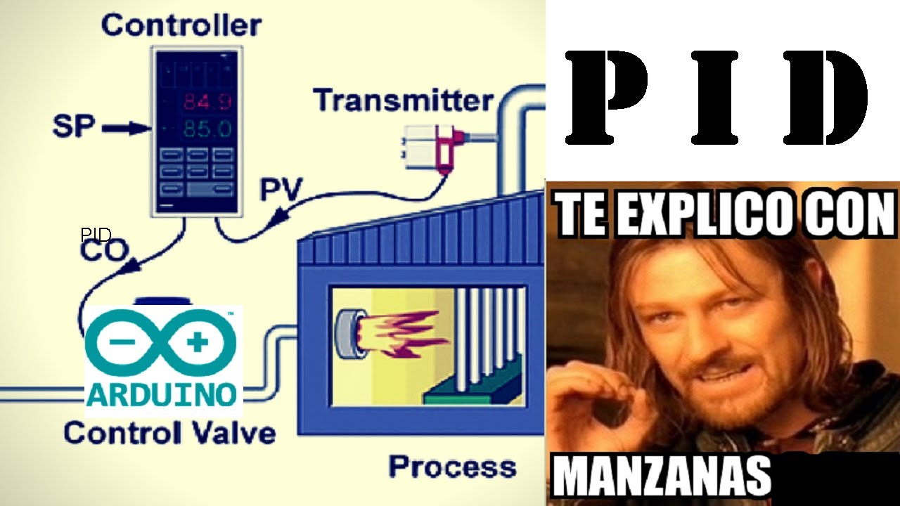
Cómo implementar un controlador PID? | PID la guía definitiva | PID paso a paso.
29.6K
Implementing a PID controller requires combining the three calculated terms using gain coefficients (Kp for proportional, Ki for integral, Kd for derivative): control_output = Kp×error + Ki×integral_error + Kd×derivative_error. These gain values must be carefully tuned for each specific system, as optimal values depend on the particular dynamics of the plant being controlled. Properly tuned PID controllers cause the measured response to converge smoothly toward the desired setpoint with minimal oscillation. The tuning process involves finding the right balance between responsiveness and stability, as overly aggressive gains can cause instability while insufficient gains result in poor performance.
Click to watch →

JMC Servo Tutorial Part 7 ► Grundlagen der PID Einstellung
20.4K
PID Regler bei JMC Servos werden schrittweise eingestellt: zuerst den Stromregelkreis (innerer Regelkreis) mit einem steilen Anfahren testen, dann den Drehzahlregelkreis, und schließlich den Positionsregelkreis; dabei sollte man die Parameter so hoch wie möglich wählen, ohne dass das System anfängt zu schwingen, und bei Schwingungen das Glied (D-Anteil) erhöhen, um das System zu dämpfen.
Click to watch →
Как сделать НАСТОЯЩИЙ сервопривод из любого мотора. Подчиненное регулирование. Робособаке быть?
468.9K
All servo systems operate on feedback control principles, comparing desired and measured positions to minimize error. PID controllers combine three components: Proportional (P) provides immediate error response, Integral (I) eliminates steady-state error, and Derivative (D) anticipates future changes to improve stability. Implementation involves summing these operations and converting to PWM signals for motor control. Position-only control has limitations: jerky movements without speed control and potential damage without torque control. Tuning requires systematic adjustment of coefficients, starting with proportional gain and adding derivative and integral components as needed.
Click to watch →
![Controlador PID via Integral del Error 💥 [Sintonia]](https://i.ytimg.com/vi_webp/GH0sjyPOztQ/maxresdefault.webp)
Controlador PID via Integral del Error 💥 [Sintonia]
7.7K
The López method (1957) provides PID tuning formulas based on the control ability factor θ/τ (range 0-1), using constants a, b, c, d to calculate Kp, Ki, Kd. The Rovira method (1969) extends this for servo control with additional constants a*, b*, c*, d*, e*, f*. Both methods substitute system parameters into these formulas to obtain controller gains. López's method tends to produce more oscillatory responses, while Rovira's is more conservative. These systematic approaches enable practical PID tuning without trial-and-error, making them valuable tools for industrial control applications.
Click to watch →
Deep Dive
Integration of encoders and feedback sensors to achieve high-precision motion control.

MOTORS -The Secret Life of Components, a series of guides for makers and designers 11
164.7K
Servo motors contain encoders with fine-line discs that sensors read to track exact rotor position. This feedback allows the motor to know its precise angular position. Integrated servo motors combine motor, controller, and encoder in a single package. They provide exceptional precision, demonstrated by maintaining position to within fractions of a millimeter, making them essential for robotics and precision automation.
Click to watch →

Apresentação de Controladores Kalatec / Xinje
2.9K
HM controllers support integration with encoders and inductive sensors for precise motion control. Encoders provide feedback on motor position and speed, while inductive sensors detect the presence or position of metallic components. The system demonstrates using these sensors to read movement data, enabling closed-loop control where the controller can adjust motor output based on actual position feedback rather than open-loop pulse counting.
Click to watch →
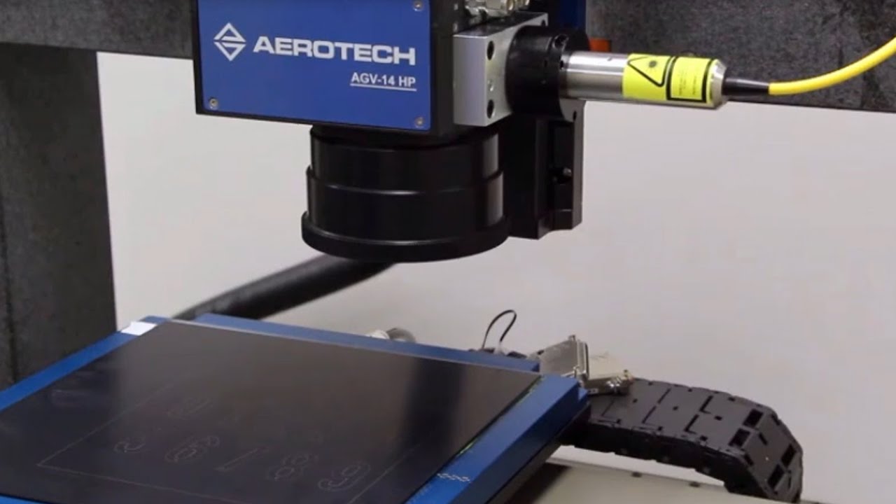
Infinite Possibilities – Easily Combining Scanner and Servo Motion
12.1K
Encoder feedback from both servos and scanners is fed directly into the motion controller at hardware level with virtually no latency. This hardwired signal allows immediate position sharing between galvo and servo systems, avoiding millisecond delays from PC-controller communication and tens or hundreds of microsecond delays from servo update rates. This real-time integration enables seamless coordination of combined motion profiles.
Click to watch →

Webinar - Motion System for Assembly Technology (ENG)
187
Precision motion control requires integration of multiple components including encoders, decoders, and control electronics. Encoder technology provides position feedback enabling closed-loop control systems that correct errors and maintain accuracy. Free axis drive technology simplifies motion control by eliminating mechanical coupling between components. The integration of these elements enables real-time monitoring, adaptive control, and comprehensive system diagnostics essential for high-precision manufacturing applications.
Click to watch →
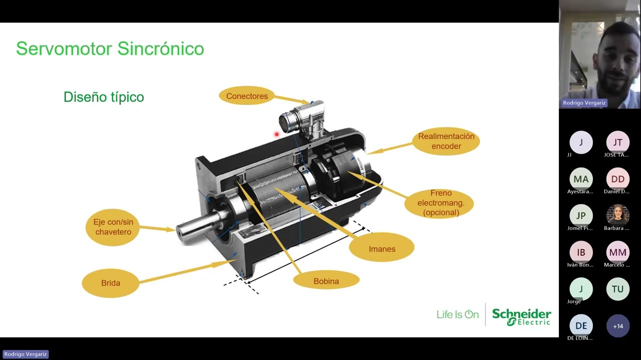
Webinar Motion Control
411
Encoders convert angular position into digital signals for closed-loop motion control. Two main types exist: incremental encoders provide relative position changes through A and B signals 90 degrees out of phase, requiring homing to establish absolute position; absolute encoders provide unique position codes for every angular location, eliminating the need for homing procedures. Advanced sine-cosine encoders output analog sine and cosine waveforms that drives interpolate to determine precise position values. Both types may include Z signals indicating complete revolutions. Encoder resolution directly impacts system precision, with higher resolutions enabling finer position control in applications like CNC machining and robotics.
Click to watch →
Deep Dive
Practical application of stepper and servo motors in CNC machinery, 3D printing, and robotics.
Power System 02 | SSC JE Previous Year Question Paper | Electrical Engineering | SSC JE 2023
20.5K
Stepper Motor receives pulse input for control, with rotor moving in discrete steps determined by step angle. Step angle formula: Step Angle = 360 / (N × R), where N is stator teeth and R is rotor teeth. Resolution = 360 / α, where α is step angle. Common step angles are 1.8, 2.5, 7.5, and 15 degrees. Rotor speed formula: Speed = α × f. Applications include 3D printers, CNC machines, and robotics. Servo Motor is a two-phase induction motor with 90-degree winding separation. Maintains constant torque from zero to full speed, can hold position without power, and quickly reverses direction. Applications include robotics, CNC machines, and automated systems.
Click to watch →
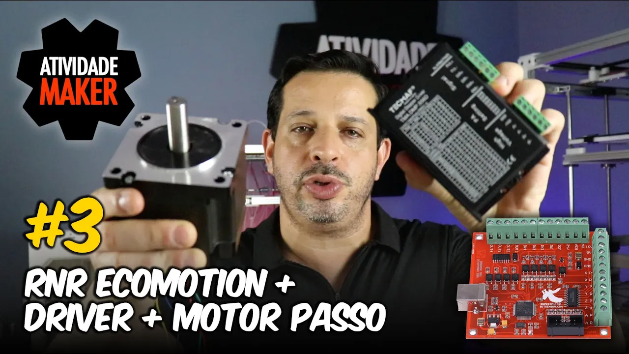
Placa CNC RNR ECOMOTION + Mach3 + Driver + Motor de Passo #3
84.2K
This video demonstrates two methods for installing stepper motor drivers on CNC controller boards: the positive signal method (connecting pulse+ and direction+ to controller outputs, with pulse- and direction- to GND) and the GND method (connecting pulse+ and direction+ to 5V, with pulse- and direction- to controller outputs). The GND method is recommended as it reduces electrical interference. The video covers connecting motor coils to the driver, configuring current settings using dip switches, and testing motor operation through Mach3 software.
Click to watch →

✅ Configurar Velocidad de Motor de Paso para CNC e Impresora 3D #8C
318.3K
To configure optimal stepper motor speed for CNC machines and 3D printers, use GRBL firmware commands ($4 for speed, $5 for acceleration, $1 for steps per mm) and systematically test by increasing speed while monitoring for step loss, vibration, or inability to stop the motor under load; the optimal speed is the highest setting where the motor can be stopped by hand pressure under load, indicating it will function reliably during actual operation.
Click to watch →

Converting a Precision Matthews Mill to CNC with MASSO | Part 1
97.4K
Servo motor systems represent a significant advancement over stepper motors for CNC applications, offering consistent torque across all operating speeds without the torque degradation that occurs in stepper motors at higher RPMs due to winding inductance. ClearPath servos integrate motors, drivers, and encoders in a single package, providing self-contained solutions with built-in feedback for step loss detection. For ball screw-driven axes, NEMA 34 electric brakes are essential to prevent axis sagging when power is off. The combination of servo motors and brakes ensures precise, repeatable positioning critical for CNC machining operations.
Click to watch →
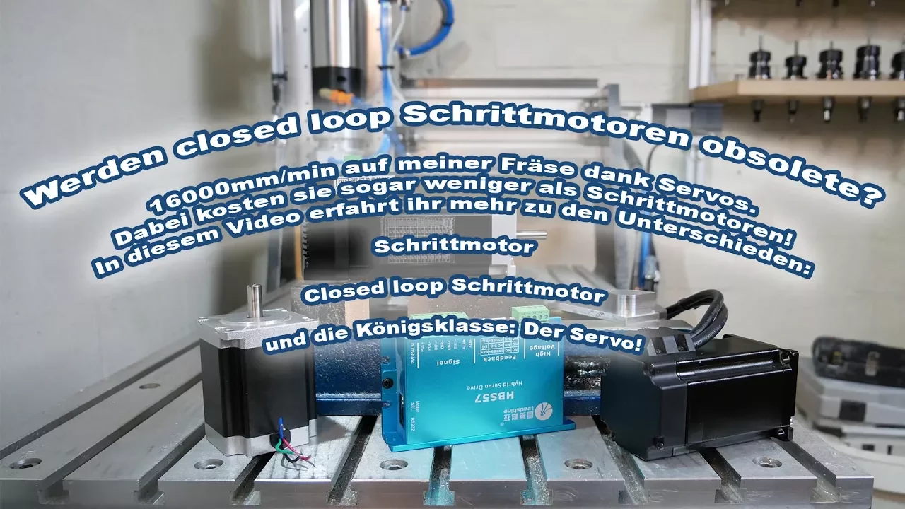
Servos für 133 Euro? mit 180W? Hier seht ihr was sie leisten können! Und was nicht ;)
149.9K
Servo motors with closed-loop feedback systems provide significantly better performance than open-loop stepper motors in CNC applications, offering superior accuracy, reduced resonance, and the ability to detect and respond to errors, while modern servo systems have become affordable enough (around 133 euros per unit) to make upgrading CNC machines economically viable.
Click to watch →
Motor Comparison
Final Verdict
Motor Comparison
0:00- 1
Steppers have slow start-up and open-loop control.
- 2
Servos excel in speed, precision, and closed-loop feedback.
- 3
Servos handle overloads better but cost more than steppers.
The Convergence of Technologies: Closed-Loop Stepper Motors (Step-Servos)
Traditional guides present a strict binary choice between simple, low-cost open-loop stepper motors and high-performance, expensive closed-loop servo motors. However, this dichotomy is increasingly outdated due to the rise of closed-loop stepper systems (often called step-servos). By adding encoder feedback to a stepper motor, these hybrid systems eliminate the classic drawbacks of traditional steppers—such as lost steps, stalls, and high heat generation—while retaining their high low-speed torque and lower cost relative to traditional brushless servos. Introducing this third category challenges the traditional 'stepper vs. servo' debate, demonstrating that modern motion control is a spectrum rather than a binary choice, and offers students a more accurate picture of current industrial engineering solutions.
Basic principles of electromagnetism and how electric motors generate torque.
The conceptual difference between open-loop and closed-loop control systems.
Fundamentals of rotational mechanics, including angular velocity, torque, and inertia.
How microcontrollers or PLCs send digital pulses to drive external hardware.
How to select and size motors for specific mechanical loads (motor sizing calculations).
Implementation and tuning of PID (Proportional-Integral-Derivative) controllers for servo systems.
Integration of encoders and feedback sensors to achieve high-precision motion control.
Practical application of stepper and servo motors in CNC machinery, 3D printing, and robotics.
147.5K views1.1Klikes2:16@ATOcom-AutomationOriginal Release: 2024-03-31
difference between steeper Motors and server Motors first the different in Star speed for steeper Motors it generally takes 200 to 400 milliseconds to start up while S Motors start several hundred times faster than that taking only a few milliseconds second they're different in accuracy the accuracy of steeper Motors depends on the number of faces and subdivision control of the steper motor driver nowadays the maximum micro step subdivision of a step motor driver can achieve up to 25,600 steps per Revolution however the accuracy of a typical Silver Motor is determined by the resolution of the encoder with the 17 digigit encoder 131,072 PES are required for the motor to complete a full rotation as such stepper Motors run sueme in terms of accuracy compared with their server counterparts these two Motors also defer in their Control Systems steer Motors don't typically employ feedback systems operating in an open loop fashion and contrast Sero Motors operate with Clos Loop control which allows direct sampling of the built-in encoder feedback signal making the more reliable than Silver Motors overload capacity is another distinguishing factor between these two motor Technologies steper Motors generally are not equipped to withstand overload so that they could lose steps at the presence of overload Sero Motors on the other hand can overcome certain overload hence better for varing load applications cost is also an important aspect to consider consider When selecting the right motor St Motors are generally more affordable and straightforward to operate making them a popular choice for many applications in comparison sub Motors tend to be more expensive and require additional components for Clos Loop control in summary server systems outperform steple Motors in many aspects though featuring more complex control but if your project requires a m solution that features simple operation a smaller price tag open look control minimal positional erors as well as other less demanding conditions St Motors will be an excellent choice visit at.com now and explore our wide range of steep Motors and Silver Motors
Up Next

53:52
Solar Concentrating Collectors: Types, Tracking & Applications
@iit
66.3K views•2008-10-24

30:32
Ultrasonic Transducers: Resonant Frequency Measurement and Horn Design
@imajeenyus42
229.9K views•2017-02-22

54:16
Polymer Environmental Degradation: Mechanisms & Stabilization
@iit
1.8K views•2012-07-10

33:39
How a Student's Question Saved a NYC Skyscraper from Collapse
@veritasium
22.8M views•2025-04-26
Related Study Plans & Knowledge Roadmaps
Structured learning paths in Engineering
engineering
Building Acoustic Levitators: Physics & Arduino
01The Physics of Sound and Standing Waves
02Piezoelectric Transducers and H-Bridge Drivers
03Arduino Programming: Generating 40 kHz Signals
+ 2 more learning modules
14h5 modules
Explore Roadmap
engineering
Building Peltier Cloud Chambers: Particle Tracks
01Cosmic Rays & Cloud Chamber Physics
02Thermoelectric Cooling (TEC) Fundamentals
03Custom Liquid-Cooling Loop Design
+ 2 more learning modules
18h5 modules
Explore Roadmap
engineering
Yagi-Uda Antennas: Modeling, Build & VNA Test
01Introduction to RF and Antenna Fundamentals
02Yagi-Uda Antenna Design Principles
03Antenna Modeling and Simulation in 4NEC2
+ 2 more learning modules
18h5 modules
Explore Roadmap
engineering
ECG Monitor Design: Op-Amps, Filters & Noise
01Electronics & Breadboard Basics
02Op-Amps and Instrumentation Amplifiers
03Bioelectricity and ECG Fundamentals
+ 2 more learning modules
18h5 modules
Explore Roadmap