












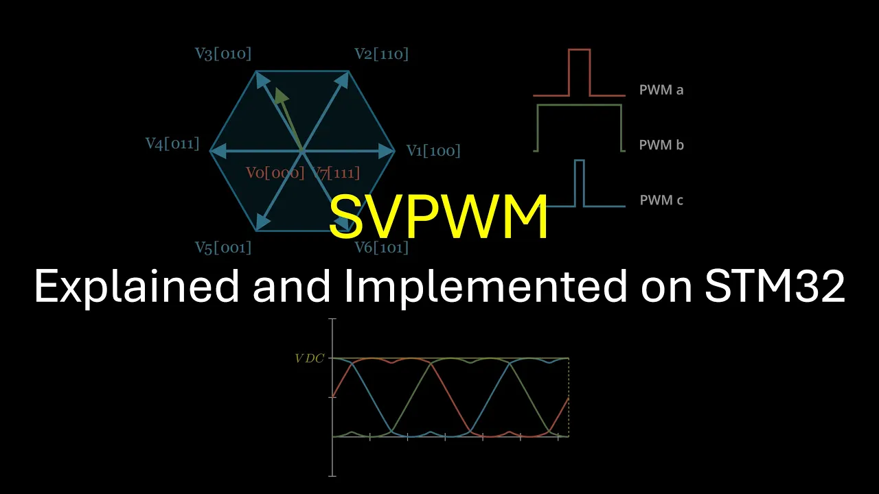







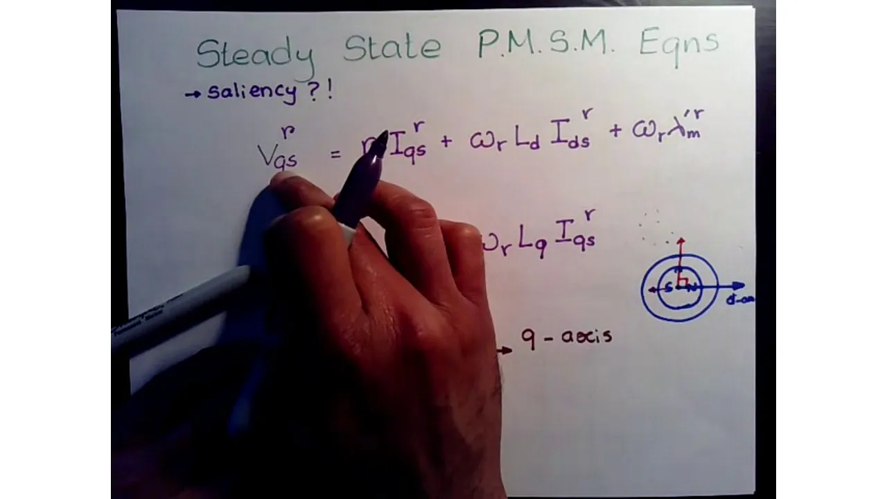

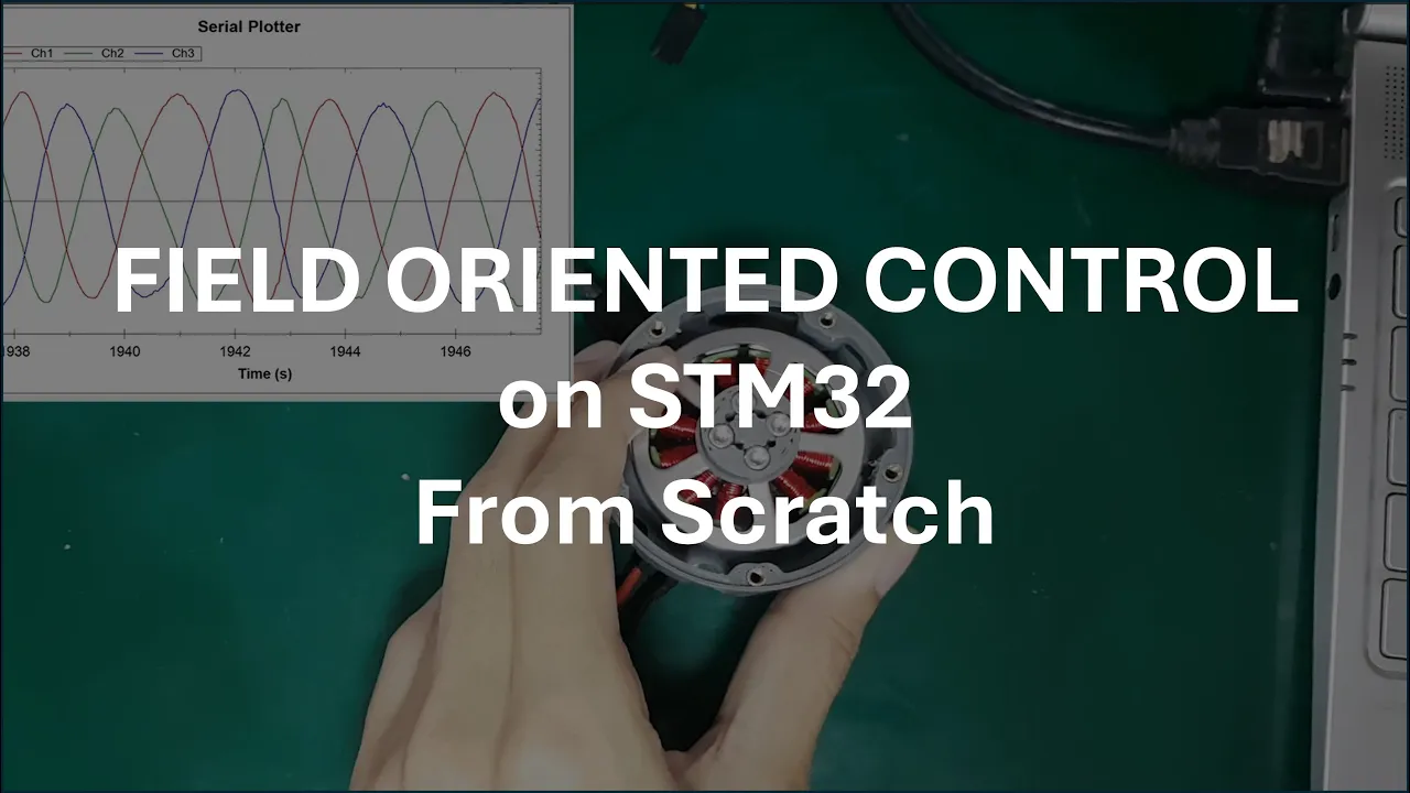


Field Oriented Control (FOC) is a sophisticated motor control technique that maximizes torque per ampere by maintaining the stator current vector at 90° to the rotor flux, achieved through a four-step process involving current measurement, error generation, voltage amplification, and PWM modulation; modern implementations use observers to estimate rotor flux angle without physical sensors, enabling sensorless control by reconstructing back EMF signals from motor currents and using angle demodulation to determine rotor position.
Field Oriented Control of Permanent Magnet Motors
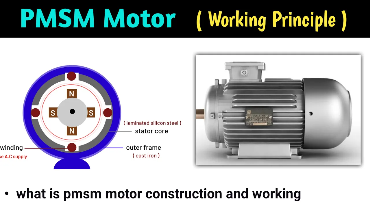
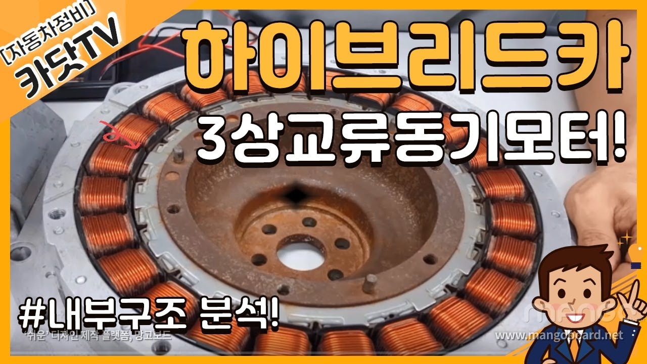
Added:Fundamental operating principles of Permanent Magnet Synchronous Motors (PMSM) and three-phase AC motor dynamics.
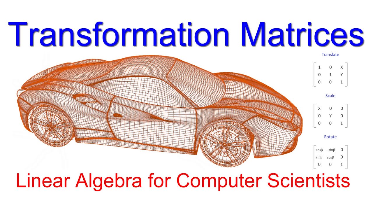
Basic linear algebra and trigonometry, particularly vector rotation and coordinate systems.
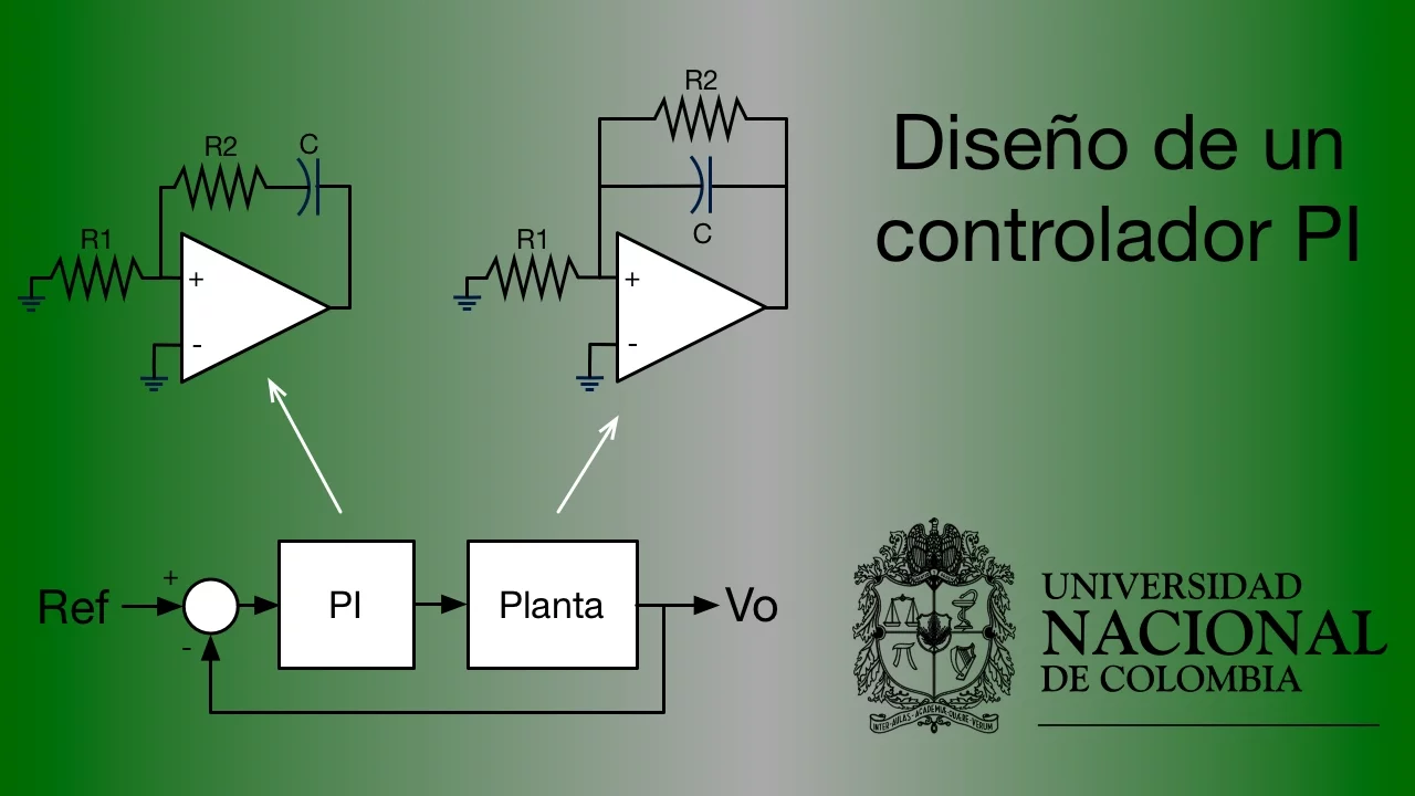
Classical control theory concepts, specifically closed-loop feedback systems and PI/PID controller design.
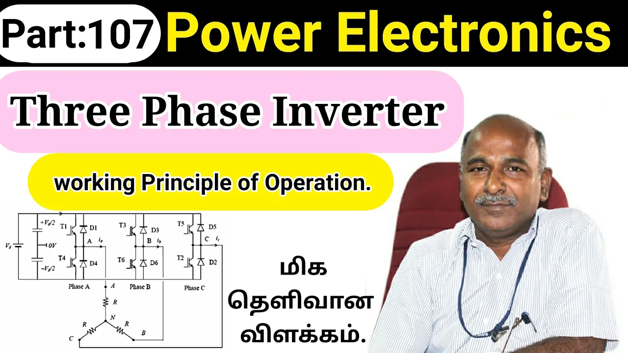
The basics of power electronics, including how three-phase inverters convert DC voltage to variable AC voltage.
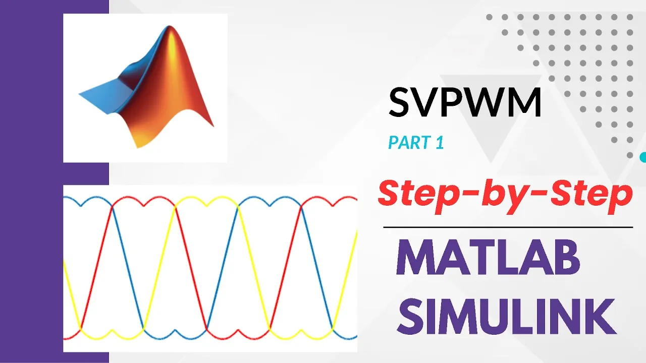
Space Vector Pulse Width Modulation (SVPWM) techniques to map FOC voltage commands to physical gate signals.
Advanced sensorless estimation algorithms, such as Sliding Mode Observers (SMO) and Extended Kalman Filters (EKF), for zero-to-low speed operation.
Field Weakening and Maximum Torque Per Ampere (MTPA) strategies to extend the speed range of PMSMs.
Practical implementation of FOC on digital signal processors (DSPs) or microcontrollers, addressing challenges like execution timing and ADC sampling synchronization.
366.6K views5.2Klikes53:43Original Release: 2012-08-29
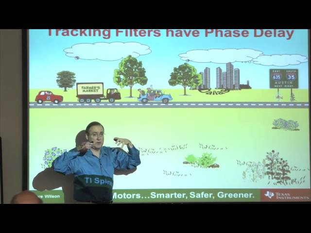
hi my name is Dave Wilson and I work for Texas Instruments for the next hour or so I'd like to talk with you about perhaps the most important motor control technique since the invention of the electric motor it's called field oriented control now it was first proposed by a researcher at Seamans named Felix blashki in the late 60s in his system he actually had flux sensors in the air gap of the machine in order to sense the flux but today the technology has evolved to the point where we don't need flux sensors in the air gap in fact we don't need any sensors at all except for the signals that the motor is providing now that's called sensorless control and we'll talk about that later in the presentation but to introduce the topic let's first take a look at how torque is controlled in a DC machine on any electrical machine in order to control the torque we must control the current now this slide might seem rather simplistic but bear with me because there's an important point that I want to make at the end of this slide first of all we're going to divide the process up into four distinct steps and the first step is we need to measure the current that's already flowing in the motor so in this case I show a shunt resistor which is actually feeding an a TOD converter so we take a sample of the current reading and then number two We compare the measured current with the desired current and generate an error signal now once we have that error signal step three is we amplify the error signal to generate a correction voltage notice that in order to control current we're actually using voltage if the current is too low we need to increase the voltage and if the current is too high we need to decrease the voltage and then finally we simply modulate the correction voltage onto the motor terminals so why is this slide so important well the reason I broke it up like this is because these four steps right here constitute the process of doing current mode control and you can picture the this as being done like by a processor where each one of these steps are done thousands or perhaps even 10 thousands of times every second the point I'm trying to make and this is the relevant Point here if you can understand these four steps then I think you're you're well on your way to understanding field oriented control in fact what we're going to see as we go through this process is that field oriented control falls under these four basic steps and you'll notice at the top of every slide that we're discussing you can take a look to see which Step we're actually on whether it's Step 1 2 3 or 4 so with that said let's take a look now at how we control torque on an AC machine with a three-phase machine we obviously have three currents to control instead of just one and if you look at those three currents on a space Vector diagram what you'll see is the addition of those three currents will actually create a current Vector with a certain magnitude and a certain angle so by controlling those three-phase currents to be just the right values we can create a current Vector to be at any angle and any magnitude that we want so the question becomes what angle should we shoot for to answer that question let's take a look at the chart in the upper right hand corner of this slide and here I've actually plotted the torque produced by a permanent magnet three-phase machine as a function of the angle between the rotor flux and that current MMF from the stator now you see that 0 degrees in other words when the current MMF Vector is right on top of the rotor Vector there's essentially zero torque but as we get out to either Plus 90 orus 90° we see that at that point we actually get the maximum amount of torque for a given amount of current in other words that's the maximum torque per amp angle so what makes sense that in most cases what we should shoot for is to try to orient our Stater current MMF Vector to be at 90° with respect to the rotor flux if I can achieve this then the torque equation at the bottom of the slide applies and that indicates that the torque on a three-phase permanent magnet machine is proportional to the product of the rotor flux times the component of the state or current Vector which is at 90° with respect to that rotor flux Vector to control the torque on the machine I don't change the angle of my state or current Vector with respect to the rotor flux I always leave that at 90° because that's where I get maximum torque per amp instead I regulate the amplitude of the state or current Vector so to do this on a digital processor the process would go something like this I'm going to get an interrupt on my processor I'll go into the interrupt service routine and the first thing I want to do is measure the rotor flux angle because once I know the angle that the rotor flux is at then it becomes simply a matter of calculating the right values for phase a phase B and phase C current to create a state or current Vector which is 90° with respect to that rotor flux angle I then apply voltages to the windings of the machine in an attempt to regulate the currents to be the desired values that I just calculated after I do that I exit the interrupt service routine and then maybe 100 microc later I get another interrupt by this time the rotor has moved to a different angle so I need to read that new angle and then recalculate my current values again I do this over and over and over and that is the process of field oriented control so let's go ahead and start the process and I'm going to measure the current or in this case the currents plural that are already flowing in the motor now I'm going to assume that my motor windings actually form an isolated load uh in this case that means that they're not connected to the motor frame or they're not connected to Earth ground they're just connected to each other and that's it so what that means is I don't need to measure all three phase currents as shown here if I know the currents that are flowing into phase a and phase B then if the circuit is isolated that means that both of those currents summed together have to equal the current that's flowing out of phase C so what I do is I take those two readings with my a TOD converter and those are just scalar values so I can figuratively speaking I can reflect them along the magnetic axes for each one of the phases as shown to the right here so I'll take the scalar reading for phase a that goes along the a magnetic axis and then the same thing for phase B now I take those two amplitudes those two values and I negate them and I reflect those along the C axis so since both A and B currents are positive that means that by definition C current must be negative now I actually have three current vectors and if I add them together I can then form the net current vector and that's the vector that I want to orient to be 90° with respect to my rotor flux so at this this point we've already completed step one and we're ready to move on to step two so step two is to take the measured currents and compare them with the desired currents and generate error signals so here I have this uh Stater current Vector that I calculated in the previous slide and the question then becomes well what is the desired current Vector is that really what I want well it depends on what the angle of the rotor flux is so if my rotor flux along this axis for example then yes perhaps that's exactly what I want because it's at 90° with respect to that but let's say that the rotor flux is actually along this axis then that means that we would want to have a commanded current Vector to be at 90° with respect to that so we actually can form an error Vector as shown here how do we correct for this well we need to regulate the input currents I a ib and IC to be just the right value so that we move the the Stater current Vector to be on the same axis as the commanded current Vector so it should be pretty obvious from the previous slide that if we're going to regulate the motor currents correctly we need to know what the angle of the rotor flux is and we can do that on a permanent magnet machine relatively easily by measuring the angle of the rotor itself that's why these machines are called synchronous Motors is because the angle of the rotor flux never changes with respect to the angle of the rotor so if I measure the angle of the rotor then I know what the angle of the rotor flux is going to be now with AC induction machines is not quite that simple because the rotor flux is sweeping across the face of the Rotor at a frequency which is equal to the slip frequency but for now let's just keep our attention focused on permanent magnet machines how do I achieve that angle of the rotor flux well I need some kind of shaft sensor which can give me really good angle resolution and there's several devices that can do that for example a resolver or an encoder are good choices for for doing this and that angle is usually taken with respect to the magnetic axis of phase a that's the way the equations have just uh traditionally been set up to work the problem with either one of these devices is that they can be very expensive so we're going to see later in the presentation how for a lot of speed control applications we can actually do away with the resolver or the encoder and do the flux angle estimation just by looking at the signals coming back from the motor so here you can see a pictoral representation of what we're trying to accomplish we measure the currents in Phase a and phase B we then add them together and then negate that sum and that actually forms the current for phase C so now we have all three currents measured in the machine and what we do is we compare those against the desired currents and how are those desired currents calculated well they are actually uh synchronized to the rotor angle by measuring the the angle of the rotor and then then from that those currents are calculated in such a way that they will generate a net current Vector which is 90° with respect to the rotor flux and when that happens it turns out that those currents will actually take the shape of sine waves so we have three current Regulators working uh in the stationary frame but it turns out that Nobody Does it this way because there's actually a better way and we'll talk about that in the next slide you may recall from your trigonometry class that in order to specify vector's magnitude and angle we need a coordinate system with only two axes not three so really we have with our three-phase machine we have a redundant phase and we can actually simplify the calculations by converting our three-phase machine into a two-phase machine so you can actually think of the machine as a two-phase machine where the coils are mounted at 90° with respect to each other so I would have a sign coil and a cosine coil now obviously we're not changing the machine at all we're just changing how we look at it it so we're going to create two axes one is the alpha axis and the other one is the beta axis and we're going to take our three-phase currents and translate those into equivalent Alpha and beta coordinates and the equations to do this are actually very simple it's just a uh you know three multiplies and uh and a subtraction and that's it so you can see here how I can use the Clark transformation to simplify the current regulation process once again I sample the phase currents for phase a and phase B and from that I can calculate phase C current once I have those three currents I use the forward Clark transformation to turn those three currents into two equivalent currents which exist on the alpha beta reference frame and then I do the regulation in that reference frame I compare those currents to the desired currents to generate correction voltages V Alpha and V beta then I use the reverse Clark transformation which I haven't talked about yet but we'll get into that in a later slide I use that to turn the V Alpha and V beta voltages into three-phase voltages that I can actually drive my machine with so you can see I've actually reduced the number of current Regulators from three to two but it turns out that Nobody Does it this way either because there's even yet a simpler way to do it and we'll talk about that coming up to introduce the next level of simplification let's take a look at this slide let's say that you're in college and you've been assigned to a design team whose job is to design an optical tracking system to track a Target that's moving on a Maro around so as the target is moving or is spinning round and round from your Vantage Point it looks like the target is actually following a sinusoidal profile and as the Maro round goes faster and faster of course that means that the frequency of that sine wave is going to increase that means you might have to design your Optical tracking system with better components higher frequency comp components because it's obviously a lot harder to track a high frequency object than it is a slower moving object so we see here that tracking a rotating object from a stationary reference frame is not a very easy task to do how can we simplify that now let's say that there's another design team that's been given the same task with one significant Advantage they're told that they can actually Mount their tracking system up on the merar round well which design team would you rather be part of obviously if you're trying to track a rotating object from that same reference frame all the sine waves and and the sign profiles they drop out of the equation and all you have now is a slower moving essentially a DC Target instead of an AC Target to track so let's apply this to our AC motor it makes a lot more sense instead of trying to regulate those currents in a stationary reference frame let's jump up on the rotor from that rotating reference frame and do the current regulation there that means that the pi Regulators that we use can actually be a lot simpler and don't have to worry about tracking nearly as fast of a Target so let's take our Alpha and beta currents and represent them in another coordinate system that's actually rotating synchronously with the rotor flux the most common orientation of this rotating reference frame is one where one of the axis is lined up directly with the rotor flux angle that's why that particular axis is called the D AIS and then the quadrature axis with respect to that is called the qais the process of doing this is referred to as the forward Park transformation and as you can see it involves a little bit more math than the forward Clark transformation now we need to take the angle of the rotor flux with respect to the a magnetic axis and we have to do some trigonometric calculations with that um it turns out that these calculations very rarely involve you know doing a tailor series expansion or something like that in most cases you just simply use a lookup table that's in memory to derive those angles but still it does require a little bit more math uh than the forward Clark transformation so here's an animation that shows the park transformation in action and what you'll see here is that under steady state conditions in other words the amplitude of the current Vector isn't changing that that will result in DC quantities on both the D and Q axis and these values are a lot easier to regulate than values that are moving sinusoidally so finally we're at the point where we're ready to regulate our currents and we see that we have our motor currents transformed into equivalent dxis and qais currents and the question now becomes well what do we want to command for the currents for the D axis and the Q axis well keep in mind we said earlier that we would like to have all of our Stater current Vector to be 90° with respect to the rotor flux that would indicate that the commanded value for the dxis current should be zero we don't want any of that current Vector to be on the dxis we want it all on the Q axis and what should we select for the commanded value of the Q axis current well that's actually the torque that we want the machine to generate for example let's consider an electric vehicle application now many people think that when you push down on the accelerator pedal that you're actually commanding speed that's not true when you push down on the accelerator pedal even with the combustion engine you're commanding torque not speed so with an electric vehicle let's say you have a potentiometer hooked up to your accelerator pedal the value off of that potentiometer it runs right here into the Q axis as as IQ current so we essentially have two current Regulators one for the dxis and one for the qais and we're now done with step two step three is that we take the error signals that we calculate ated in the previous slide both for the D and Q axis and we amplify them and in this case we show Pi Regulators being used to do that function it turns out that due to the nature of the poles in the transfer function for most current Regulators that we don't need additional phase compensation so we don't need like a PID regulator unless of course your sampling frequency is really low or there's other things in your system that are causing phase delay but in in most cases a pi regulator is sufficient to do that so what we're doing in this case is we're generating two correction voltages now one for the dxis and one for the qais once we finish this step we're ready to proceed to the fourth and final step if you've made it this far congratulations now just hang in there for a little bit more because we're almost done step four is to take these two voltages and apply them to the motor terminals but wait a minute we can't apply VD and VQ directly to the motor terminals for a couple of reasons number one these values exist on a rotating reference frame if we're going to apply them to the Stater coils we need to transform those back down to a stationary reference frame and then the second reason is we only have two values VD and VQ we need three values because remember we have a three-phase machine so there's a couple of steps that we got to go through yet and the first one is the reverse Park transformation now this is the one that gets you down off of that rotating reference frame back into a stationary frame so we're going to turn VD and VQ into V Alpha and V beta which are a stationary reference frame and the equations required to do this look very similar to what we Ed to get up onto the rotating reference frame we have the same cosine and S calculations that need to be done and once again we can use a lookup table just like we did uh in the forward Park transformation so here's an animation that shows this process and once again we see that for steady state VD and VQ values that that translates into sinusoidal Alpha and beta coordinate values so once we have V Alpha and V beta we see that they form a voltage vector and the goal is to come up with three equivalent voltages on a three-phase reference frame which will generate exactly that same voltage vector and this is shown here as the reverse Clark transformation you can see that the equations are very similar to the forward clar transformation there's a few more multiplies and additions but still it's something that can be quickly calculated by most processors once I have these three voltages I simply scale them appropriately and apply them to my modulator whether it be a pwm module or some kind of space Vector algorithm or whatever and that's it we'll see that over time under steady state conditions that these three voltages will turn into three phase sine waves that are phase shifted by 120° at that point I fall through the bottom of my interupt service routine and then I wait for the next interrupt where I go do the whole process over again and uh by that time the rotor has moved to a slightly different angle my currents are a little bit different hopefully the currents are different in a way that they've moved closer to the desired values that I want and then I just repeat the whole process over again so here you can see how field oriented control is commonly done once again I sample the a phase current and the b-phase current I add them together and then negate the result to achieve the c-phase current now I've taken the liberty of lumping the Clark Park transforms together for clarity sake so I take IIA IB and IC and I transform those into ID and IQ and those are essentially DC values so I'm doing the regulation actually in a reference frame if you look at it on a scope where those values are not changing ing very rapidly at all at least under steady state conditions so I do the regulation there to generate VD and VQ correction voltages I then run back through the reverse Clark Park transforms to generate my phase voltages to drive the machine with here we see a typical example of a field oriented control system the top block contains all of the Power Electronics and the bottom block is actually one of our processors that's the 280 3x device commonly known as the piccolo and let's talk about a couple of things on this part that I think are relevant to this application first of all you'll notice that the signals from the quadrature encoder mounted on the motor shaft are decoded directly by a module on the Picolo part so there's no reason for an external decoder to sit out there between the encoder and the processor that's all done on the part where we actually take the quadrature signals and decode those into a position variable the next thing to not notice is that the pwm module actually has a sync pulse which is used to trigger the 12-bit ad converter and this is important because you need to acquire your current readings at exactly the right spot within the pwm cycle and the timing can be so critical that you can't rely on software in many cases to do that for you so having a sync pulse where you can actually sample the currents at exactly the optimum value in the pwm cycle is very important to motor applications now if you look inside the processor block some of the individual blocks are red and some of them are purple it turns out that the hardware modules inside the processor are shown in red and the software blocks are shown in purple and if you look at the way that this field oriented control algorithm is hooked up it's actually part of a cascaded control Loop where we have a speed Loop wrapped around it so what we're doing is we're taking the actual speed uh comparing it against the commanded speed and generating an error signal and that becomes the torque command for the field oriented control controller so if we're going too fast for example then we need to have less torque or if we're going too slow we need more torque so this is actually a very common way that this is done now Texas Instruments has several reference designs available that do field oriented control on the piccolo processor we have reference designs for permanent magnet synchronous Motors and also for AC induction Motors so if that's something you'd be interested in please visit our website uh www.ti.com motor control and you can have access to those reference designs another great application for field oriented control which is actually gaining in popularity is electric power steering and what we have is a torsion bar mounted in the steering column which generates a different angle from one end of the bar to the other end of the bar as a function of how much torque is being applied by the steering wheel so that torque signal is applied to a processor which is implementing field oriented control and that's used to drive a permanent magnet synchronous motor which is hooked up either to uh the rack and pinion directly or in the column of the steering wheel to provide torque assist when you turn the steering wheel now as I mentioned earlier using a resolver or an encoder on the motor shaft to get rotor flux angle information is very expensive but we've also seen as we've gone through the field oriented Control process that having that rotor flux angle is absolutely a critical piece if we're going to do field orientation control so we need to find another way to get that information without having to have a shaft sensor and that serves as a launching point for a discussion on model-based filtering so what I have here is I have a process which is generating some kind of signal unfortunately I can't get to that signal because it's buried down inside the machine or it's contaminated with noise the only measurement that I can achieve is the signal after it's been contaminated with the noise so what I can do is I can build a mathematical model model of my process and generate an estimate of what I think that signal should look like I then compare it to the measurement generate an error signal and that error signal is used to correct my mathematical model so that on the next iteration I can generate an estimate that should be closer to my desired signal one of the simplest instantiations of this concept is something called the tracking filter or maybe you know it by a different name the alpha beta filter and this filter really works best when you're you're trying to process a low past signal in the presence of broadband noise this particular filter consists of two cascaded integrators where the second integrator is actually making an estimate of what we think the signal should be so you can see the measurement coming in this is the one that has the noise plus the signal on it I compare that to my estimate and generate an error signal which then goes back and biases up the inputs of those integrators by two amplification factors which are the alpha and beta data blocks so if I want really good tracking performance out of this filter I can dial up Alpha and beta so that they're high values unfortunately that means I'm also going to be tracking more of the noise as well if I want more filtering I can bring those levels down and get better filtering so it really is a trade-off of good filtering versus good tracking now not long ago I was doing some modeling with the tracking filter and I wanted to put it in a form that could be processed by mathcad so I went through and and twisted the equations and what I came up with was the form that you see before you here and what I realized at that point was that the tracking filter was nothing more than a simple second order infinite impulse response filter well you can imagine my disappointment because I had always thought that the tracking filter was something rather significant or something special and here come to find out it's nothing more than a simple low pass second order I filter but as I thought about it some more I realized why we like to represent this filter as two cascaded integrators and you can see that in the next slide once again we see the tracking filter represented in the cascaded integrator form and what we see is that by representing the filter in this format it actually produces the derivatives of my controlled variable for me for example let's say that I'm trying to track a measured position that means that the output of my second integrator is going to Servo in to the estimated position now if my filter is operating with relatively low error and the output of that integrator is the measured position then it forces the input to that integrator to be the velocity of the system now that's really cool it actually morphs the signal to become the velocity signal and if that is the output of the first integrator stage and again we're operating with relatively low error then it causes the input to the first integ stage to be the system acceleration so by representing the tracking filter in this format I get a lot of useful signals out of it that represent valuable things in my system now how cool is that well despite how Nifty the tracking filter is it does suffer from one rather serious problem and that is since it's basically a low pass filter then it exhibits phase delay just like all low pass filters do in other words if it's tracking a particular signal it can't start responding to changes in that signal until those changes actually occur and this is a problem to illustrate what I'm talking about let's take a look at this animation so you're going to be in the red car and you're following this truck so your job as a tracking filter is to track the position of the bumper of that truck and and maintain that distance between your vehicle and the truck unfortunately you can't see through to the traffic in front of the truck all you can do is just track the position of that bumper so even though the traffic ahead of the truck may be slowing down you can't respond to any of those changes until the truck itself actually puts on its brakes at which point there's going to be a delay while you put on your brakes and as a result of that maybe some bad things are going to happen so let's rewind the scenario and this time instead of following a truck that you can't see the traffic ahead of it you're going to be following a car so you're still trying to track the position of the rear bumper of the car ahead of you but now you have an additional piece of information you can see the signal that is stimulating the system that you're trying to track in other words you can see the traffic conditions up ahead of the car and knowing something about how that car will respond to that perturbation you can actually simulate that response and therefore minimize or completely eliminate the phase delay of your response in control systems this effect is called called feed forward compensation in other words you're feeding forward some of the input signal of the system that you're trying to track in order to minimize phase DeLay So let's take a look at the structure of our tracking filter again but this time we're going to add a feed forward component so here we can see a tracking filter that's used to model the mechanics of a system that's used in a Servo application and just like we saw on the previous Slide the same signal that's stimulating our control system is also fed into the model of our tracking filter as a feed forward signal now when you do this the tracking filter goes by a different name it's now called an observer and observers are used very frequently in motor control systems where you want to minimize or completely eliminate the estimation lag of your tracking filter so let's take a look at an example of how an observer can actually do something useful for you in a control system now in this particular example example the output position of the servo system was measured with an encoder and with any position Servo system you also need to measure velocity in order to make your system stable so how do you get velocity information off of an encoder signal well one of the easiest ways to do it is to measure how many encoder counts occur over a specified period of time but the problem is what do you do when the motor's going very very slowly in most cases you want the time interval to be the sampling interval of your control Loop so when the motor's going really slow you end up with a situation where you may only get one encoder count per interval or two encoder counts per interval or maybe zero encoder counts per that interval so your velocity signal has become extremely quantized and if this is the signal you're trying to measure you can think of it as being contaminated with quantization noise you really don't have access to the velocity signal directly you can only get the reading after it's been contaminated with this quantization effect but have no fear because the Observer can create that velocity variable for you by forcing the output of the Observer to track the servo position in other words the encoder count value it forces that input to the last integrator stage to morph into the velocity signal and that has as much resolution as you want it to have so let's take a look at a simulation example where in one case we derive the velocity signal from the Del Del encoder count values and in the other case we derive the velocity signal from an observer this slide shows the simulated position velocity and currents of a Servo system where at tals 5 milliseconds I have commanded a step change of one revolution which is 2,000 encoder counts in particular take a look at the velocity signal so you can actually see what the actual velocity is that's the cyan colored uh graph in the middle there but look at the difference between the velocity which has been reconstructed from the encoder and also the velocity that's been reconstructed from The Observer notice how much smoother The Observer velocity variable is and especially when you get out into the tail end of the movement where I'm not going very fast you can actually see the encoder quantization problem that I was referring to and when you feed the output of your velocity Loop to the input of your current Loop look at the current perturbations that that causes when you use the signal reconstructed from the encoder there's lots of noise on that signal and actually if you've done anything with encoders you probably heard this effect before it sounds like a scraping noise or something on your motor as it's you know moving very very slowly and again take a look at the current waveform when the velocity is reconstructed from The Observer it looks much smoother and that results in much quieter operation of your motor this slide shows the actual Observer that I used in that simulation and the topology of this Observer comes from some of the work that's been done at the University of Wisconsin in Madison so you can see that the output position of my Servo the POS _ vo variable is fed back to the input side over here where it's compared to the encoder counts that generates an error signal which is then fed into a pi control Loop and this is actually the negative feedback part of the Observer and that's used to correct for any unforeseen pertubations to the system that aren't accounted for changes in the input control signal so for example uh any torque pertubations or things that couldn't be accounted for that's actually handled by the feedback path here and then you also see the feed forward path now this is the input signal coming into the Observer which is my current waveform and again that feed forward path is included to minimize the phase delay of the Observer tracking performance so let's get back to our original question and that is how can can we use an observer to get rid of the shaft sensor so that I can actually use an observer to measure the angle of the rotor flux so I've got a three-phase machine here and let's assume that I've already done a Clark transformation on it so I've essentially turned it into a two-phase machine where I now have a s coil and a cosine coil so look at this circuit diagram right here this circuit is actually common to both the S and cosine coils and if I write the voltage expression for both of those coils it's actually this Matrix expression which is shown right here and all this says is that basically the voltage which is applied to any one of those coils is equal to the sum of all the voltages around the loop of those coils so let's just take the alpha coil for example that's the top variable V sub Alpha is equal to the IR voltage drop across that stator resistor plus ldt where p is my differential operator in this case plus another term which is the back EMF component of my machine and that's basically proportional to a a back EMF constant times the speed that the machine is going times either this s or cosine term right here so in this expression where do you see anything related to shaft angle well it turns out it's actually in the back EMF signal you can see it's s of theta or cosine of theta that's my angle information that's what I need to somehow extract but unfortunately the back EMF source is buried deep down inside the motor I'd love to be able to just stick a voltage Probe on it and get that signal directly but I can't so I need to use an observer to extract that signal for me so here's how you make a back EMF Observer I'm going to start by reproducing the Stater circuit here for one of the coils and what I want to do is I want to find the the equation which would Define what the current is flowing through this coil so I can basically represent that as a steady state term which is shown here times the transient term effect which is shown here and if I actually model that if I create a block model of how to implement this it's basically taking my input voltage subtracting my backf voltage which by the way I don't know what that is yet but nonetheless let's include it here for now once I have that difference then I divide by my Stater resistance and then I run it through a single pole low pass filter so that's actually how I would represent this equation so let's take this block and let's copy it up here now you notice that my resistance variable has a hat over it that means that's an estimated variable that's my estimate of what I think the Stater resistance is keep in mind that this motor is heating up and cooling down so its resistance is changing all over the the place so what I'm entering here is basically a value that I had measured uh previous at some time in the past and then I'm going to have a digital low pass filter and I'll show you how to implement that in just a second so what comes out of that is my estimate of what I think the current should be now keep in mind that I can actually measure the current in this coil what I can do is take my three-phase current measurements and then do a forward Clark transformation on those and get I sub Alpha and I sub beta so once I have that value I'm going to compare my estimate of my current with the actual measurement that I've taken and generate an error signal from that I'm going to then take that error signal and gain it up through a pi control Loop and then I'm going to invert that signal uh the reason for that will become apparent in just a second so now that I have that output what do I do with it now watch this I'm going to take that output and I'm going to wrap it back around into this input to force it to become the missing back EMF variable now you see why I needed to multiply that term by a minus one because if I didn't I would have positive feedback through my whole Loop instead of negative feedback so here's how it works since this is a closed loop system if I can make my gain high enough in my closed loop system I should be able to drive this error term to zero or pretty close to zero what does that mean that would mean that my estimate of my current is actually equal to the real value that I measured but the only way that that could happen would be if the output signal actually turns into the back EMF signal so you see it actually morphs that output into the back EMF signal it's pretty clever so here's a simulation that I put together showing how you build a back EMF Observer and it actually consists of four blocks here and we'll go over these individually this block down here at the bottom that is my estimator uh where I'm actually trying to estimate what I think the motor current should be uh this is my actual motor phase and from the output of that I actually do have a measurement of the actual motor current in that phase uh this block over here that is my regulator you can actually see the pi uh components in here and then over here this block right here is my power stage and that's where I'm doing my PW mod modulation so let's actually zoom up on some of these and and take a look at some of this stuff and you can hopefully see it a little bit better here we go so here's the voltage coming into my motor phase it's got a series resistance it's got a series inductance and then here's my back EMF generator now this is what I'm trying to figure out now I know what this is because I'm the one that programmed the simulation but the rest of my circuit doesn't know what this is and of course the goal will be to see how well um my simulation can reconstruct what this signal is and then the output of this block all I'm doing is creating a voltage source which is a function of what the current is flowing through uh this resistor right here R1 so that's being output right here as the actual motor current um let's go down below here and here's my singlephase motor model so here I have my voltage which I'm applying to the input of the winding and then this is the input for the back kmf which I don't know what it is but uh that actually would get subtracted off from the input voltage to my winding and then that goes through a low pass filter just like I talked about earlier and this is the way I create the low pass filter it actually has an integrator uh inside of this it's a digital integrator and all of the digital components are driven by this sample clock and that's uh shown right here uh this is actually programmed to work right now with a sampling frequency of 10 khz so that sample clock is a it's just a pulse generator that feeds all of my digital control blocks like my uh you know my sampling hold my Z to the minus1 terms uh things like that uh let's move up here now here's the input voltage that I actually do want to drive the motor winding with and this is just a sine wave that's running at uh a variable called freak or frequency and that's right now set to 60 htz and I'm going to apply that then to my power stage uh where it gets modulated so then I'll just just have a pwm signal with a low frequency uh modulation on it of 60 HZ that I'll be applying to this voltage input of the winding and then the last piece we want to look at here this is the pi regulator so I take the actual current that I've measured I compare it to my input or compare it to the current that I've estimated uh subtract the two generate an error signal and then you can see it goes right into the pi control Loop this is the I term on the top this this is the P term on the bottom those two outputs get summed and then like I said I have to negate it otherwise I end up with positive feedback so let's hook all this up and if I do it right it should actually um simulate that back EMF signal so my voltage input I'm going to feed that down to the input of my model here there we go and I'm also going to take that and Supply it to my pwm module so that I can actually create a pwm signal to drive my my power stage right here and then the output of my power stage I'm going to take that and run it into my voltage input on my motor coil and then this is my estimate or no this is my actual current that I've measured so I'll feed that into the reference input here and then I'll take my estimate of the motor current I'm going to feed that in right on the other side here and then the last piece that I have to hook up is to take this output which I'm hoping is going to morph into the back EMF signal and wrap that back around to this input like we talked about earlier okay so if I've done everything correctly uh let's fire this up and see what happens so when I hit run you can see my model servos in on the actual back EMF signal very very quickly and then immediately it's uh tracking it so this stuff really does work let me go ahead and stop this here and you can see just how well that my model is tracking this uh mystery backf signal right here you know I've tried all kinds of waveforms I've tried square waves I've tried triangle waves and again depending on what the gain that you have set in your Pi Loop uh it'll track just about any kind of waveform so again this stuff uh really does work it's not black magic as incredible as the Observer is we're not out of the woods yet all we've done is recreate one of the the back EMF signals and remember what we started out to do was to try to find the angle of the rotor flux so this slide shows the whole process of how we use two back MF observers to do that the top circuit is for the alpha BMF signal and then the bottom circuit is for the beta backf signal and then we have those two signals one is a sine wave one is a cosine wave we Supply those to this output block right here which is an angle Dem modulator and what pops out on the output of that thing is an estimate of the angle of the rotor shaft and from that I can determine what the angle of the rotor flux is so you can see we went through an awful lot of steps just to get that angle of the rotor flux and then once we have that we can proceed with the rest of our steps in field oriented control just like we talked about earlier step two step three step four and so on so getting that angle is a very very big part of this whole process here's a simulation of the previous slide showing both back EMF observers plus the angle Dem modulator so let's just start over here um uh this right here is my three-phase power stage so I have VA VB and VC so I'm actually creating uh pwms that I'm driving all three of my motor windings with and then you can actually see those here here's phase a phase B and phase C so what I'm doing is I'm essentially sampling the phase a and phase B currents and then I run through the forward Clark transformation right here using all three currents and right here I create I sub Alpha and I sub beta so this right here whole block this is my back EMF Observer for the alpha circuit and then here's the back EMF Observer for the beta circuit the outputs over here are my estimates of the actual back EMF signals and again I'm keeping those a mystery uh to the rest of the simulation so it's up to The Observers to try to figure out what those signals are once they've been transformed into um a two-phase coordinate system then I have those two variables I feed them both into my angle demodulator down here and let's just uh pop this open real quick we can take a look at it so you can get a better idea of what this is so again here's the angle Dem modulation um I'm kind of doing a hoding operation by mapping the output back and multiplying the sign term by the cosine of the estimate on the output and then vice versa the cosine term by the sign of the estimate on the output so this uh this is a two-stage back EMF Observer it has two integrated two integrators in it so it's second order and this is my estimate of my angle this is what I think the angle is and of course if that's the angle and that's the output of this integrator then that means that this variable on the input of the integrator has to be my frequency so I can actually get a very good estimate of what the frequency of my system is as well now I know what the actual angle is because I know what frequency that the back EMF signals are running at and I can actually multiply that over time to get an estimate or actually to get the actual angle value I compare that to my estimate of the angle value and then I can generate an angle error which I'm going to plot to see how well my whole system is actually following that real angle so let's go ahead and back out of this and I'm going to start this thing running and let me Zoom this up right here what you see on the top are that's four waveforms those are the true Alpha and beta back EMF signals and on right on top of those are my estimates of the back EMF signal so you can see it's tracking very very well the bottom plot right here this is actually showing that I start off with an error of Min -4° uh it then jumps up to 8 deg but then it starts Sero servoing right in to the actual angle and then you can see the frequency estimate which is the variable right before that last integrator uh going right into to 60 HZ so I have a nice filtered version of my frequency as well now if we let this thing run a little bit longer actually at 50 milliseconds I change my Stater resistor without telling the Observer uh what happened so I'm actually uh estimating my signals with the wrong value of my Stater resistance and you can see that my Observer now can't follow the backf signal quite as good and as a result of that it does result in an angle shift so that's what you have to watch out for is when your parameters change and you don't know about it you start getting wrong answers for your angle estimate and then right at 100 milliseconds I changed the resistance by a factor of two in the other direction so at 50 milliseconds it's a factor of two in one direction and then a factor of two in the other direction at 100 milliseconds and you can see once again that that does cause another shift in my in my estimate so once again we can see that this stuff really does work and I would encourage you again if you get a chance uh to try to build one of these or play around with them they're really a lot of fun to experiment with ti has a very interesting reference design where we do sensorless field oriented control on two permanent magnet synchronous Motors at the same time and that's why this slide right here is showing the processor that does this is called the piccolo and I've already talked about that or alluded to that in this presentation earlier um we actually use something called a sliding mode Observer it's a little bit different than the one that I discussed here but basically it does the same thing we're trying to estimate what the angle of that rotor flux is now here's what I find to be fascinating about this reference design we are controlling both Motors using sensorless field oriented control and the sampling frequency for both of those algorithms are running at 10 kilohertz per motor yet the combined bandwidth required for both of those algorithms for both axes never exceeds 50% of the cpu's bandwidth capability I mean that's just amazing that shows exactly how powerful the piccolo is in doing algorithms like field oriented control and again we have enough pwm on it to control both Motors we actually have 14 motor control pwm which include Deadtime and all that other good stuff that you like to see when you're controlling a motor here's a slide showing the road map for R c2000 family of products and you can see that the road map is actually split into two distinct Parts on the bottom end we actually have the piccolo series that I was talking about that's the 282x and the 280 3x devices and these are you know focused more at the lower cost uh 40 to 60 mips kind of performance ranges and again like I've already Illustrated that that's plenty good enough to do a field oriented control on most Motors but if your application actually requires more processing power then you might want to consider the 28 33x family which is 150 mips and 300 megaflops these are floating Point processors or even higher than that is the 28 34x family these are 300 mips 600 mlop machines so you can see here that TI has a wide range of solutions and there's a pretty good chance that your application is going to be covered by one of these products here you can see a more complete list of some of the reference designs that we've generated for motor control and I'm not going to take your time now by going through all of these but I just wanted to make you aware that these exist if you'd like more information on these or other reference designs again please visit our motor control website it's www.ti.com slm control well we've reached the end of our presentation and I really do appreciate you spending the last hour or so with me as I've talked about field oriented control and some of the solutions that TI has to implement this technology you know when I think about all of the different topics in motor control I think that field oriented control is perhaps my favorite and I hope that you've enjoyed it as much as I do if you need to get a hold of me please uh see the information at the bottom of the slide my email is Dave Wilson ti.com or you can call me at the number that's listed there again thanks for your attention and I hope to see you in another seminar real soon
Up Next

14:29
Microbial Fuel Cells: Voltage Testing & Assembly | MFC Series
@callmeastrogirl9707
405 views•2021-05-23

30:32
Ultrasonic Transducers: Resonant Frequency Measurement and Horn Design
@imajeenyus42
229.9K views•2017-02-22

16:00
Using Low-Cost Transducers for Ultrasonic Sensing Applications
@TexasInstruments
72.8K views•2015-06-18

33:39
How a Student's Question Saved a NYC Skyscraper from Collapse
@veritasium
22.8M views•2025-04-26
Related Study Plans & Knowledge Roadmaps
Structured learning paths in Engineering
engineering
Building Acoustic Levitators: Physics & Arduino
01The Physics of Sound and Standing Waves
02Piezoelectric Transducers and H-Bridge Drivers
03Arduino Programming: Generating 40 kHz Signals
+ 2 more learning modules
14h5 modules
Explore Roadmap
engineering
Building Peltier Cloud Chambers: Particle Tracks
01Cosmic Rays & Cloud Chamber Physics
02Thermoelectric Cooling (TEC) Fundamentals
03Custom Liquid-Cooling Loop Design
+ 2 more learning modules
18h5 modules
Explore Roadmap
engineering
Yagi-Uda Antennas: Modeling, Build & VNA Test
01Introduction to RF and Antenna Fundamentals
02Yagi-Uda Antenna Design Principles
03Antenna Modeling and Simulation in 4NEC2
+ 2 more learning modules
18h5 modules
Explore Roadmap
engineering
ECG Monitor Design: Op-Amps, Filters & Noise
01Electronics & Breadboard Basics
02Op-Amps and Instrumentation Amplifiers
03Bioelectricity and ECG Fundamentals
+ 2 more learning modules
18h5 modules
Explore Roadmap