




![Termodinámica. TODO lo que DEBES SABER de la ECUACIÓN DE ESTADO [ENTRA Y APRENDE RÁPIDO Y FÁCIL]](https://i.ytimg.com/vi_webp/8nWb0zxsRew/maxresdefault.webp)


![[서울대 나용수교수님] 플라즈마 기초 3강 Single Particle Motions 1 Gyro Motion, ExB drift](https://i.ytimg.com/vi_webp/aa59FYImRPQ/maxresdefault.webp)









![BRICS Astronomy Workshop [DAY 3 - Afternoon]](https://i.ytimg.com/vi/w5DYhNIo4Gw/maxresdefault.jpg)



![[플라즈마 Kinetic Theory] Lecture 11-b. POSTECH 윤건수교수님](https://i.ytimg.com/vi/RE2N4Z9WQx4/sddefault.jpg)
![[핵융합과 플라즈마] 3.3. 6차원 위상공간 유체 (플라즈마의 키네틱 이론)](https://i.ytimg.com/vi/72tUSomExks/maxresdefault.jpg)

This lecture introduces the fundamental fluid equations for plasma physics, including density conservation (∂n/∂t + ∇·(nV) = 0), momentum conservation (mn(∂V/∂t + V·∇V) = nq(E + V×B) - ∇P), and an equation of state with no entropy production (∂(P/ρ^γ)/∂t = 0). The key insight is that in magnetically confined plasmas, the perpendicular momentum balance yields the E×B drift and diamagnetic current J_perpendicular = (B × ∇P_total)/B², which creates a magnetic field opposing the applied field—a phenomenon arising from the collective gyro-motion of particles in the magnetic field.
Plasma Fluid Equations | Magnetohydrodynamics Basics
Added:Fundamentals of classical electromagnetism, particularly Maxwell's equations and the Lorentz force.
Basic fluid dynamics principles, including the Navier-Stokes equations and fluid conservation laws (mass, momentum, and energy).
Thermodynamic concepts such as the ideal gas law, pressure tensors, and isothermal/adiabatic state equations.
Introductory plasma physics, including single-particle motion (gyromotion, drift velocities) and the concept of collective behavior.
Analysis of MHD waves, such as Alfvén waves and magnetosonic waves.
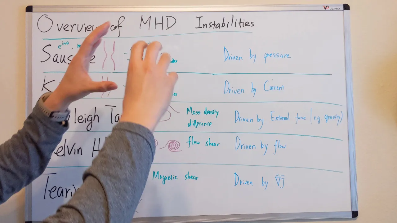
Plasma macroscopic instabilities, including Rayleigh-Taylor, kink, and sausage instabilities.
Magnetic confinement fusion principles and applications in devices like Tokamaks and Stellarators.
Astrophysical and space plasma phenomena, including solar winds, magnetospheres, and magnetic reconnection.
Kinetic theory of plasmas (Vlasov and Fokker-Planck equations) for regimes where fluid approximations break down.
6.4K views55likes49:41Original Release: 2015-12-24
okay today what we want to talk about is again a little more about plasmas are a fluid or at least the kind of description that we're going to use to try to describe plasmas as a fluid so uh let's title our things here what we're doing again uh plasmas as a fluid now some sort of uh General observations let's say uh let me remind you of a couple first is that in this plasma uh we have two species electrons and ions typically electrons and protons and so in general we can expect that the electron temperature does not equal the ion temperature and because of that um we're going to need uh usually uh going to need two species equations for uh fluid equations for two species namely electrons and ions now uh sometimes we'll be able to add them together add electrons and ions together and they all act as one fluid in which case they would be uh we would call that Magneto hydrodynamics or fluid like or almost like navier Stokes equations or something like that okay the second comment is that the force field we want to consider which will act upon uh both ions and electrons individually and then also on um on the fluid of a of a whole sequence of them uh is is from basically the electric field and the magnetic field and of course it is then the uh lorence force that is to say force is equal to Q uh e plus v crossb and we're going to have that lorence Force both on each individual particle and on all of the particles and somehow and we want to construct a fluid description hence we put them all together and how does the whole fluid act we'll talk about that in a minute and we basically want to to use the simplest fluid description we can have and for that what we will basically do um is to discuss uh therefore we'll use density and momentum conservation equations but we will for Simplicity uh we will assume that there's no heat transport or entropy production on the time scale of Interest I'll be specific about this in a moment um and also uh that there's no temperature gradient or anything like that so basically we'll set uh T equals a constant and grad T is equal to zero and um to emphasize you might say the difference from a plasma from uh regular um fluids we will neglect all dissipative effects so uh neglect dissipative effects these would be you know due to kulum collisions uh be heat flows uh um various types of entropy production neglect dissipative effects um and so we'll be treating effectively a collisionless uh plasma that is to say that our frequency uh is much great frequency for processes of interest is much greater than the Collision time and for Omega you can always just think of uh d by DT some time uh time derivative of say the density how fast it oscillates how fast it changes or something like that and hence on because we're neglecting dissipative effects there will be no entropy production on the time scale elist uh this is true for most of what we talk about um but in some cases we will have a little bit of entropy production uh because of various uh processes namely when we get into diffusion and resistivity okay so with this uh comment uh what we want to do now is talk about uh fluid equations um that we want to construct I guess is the best way to say it but before doing that I need to give you some definitions in terms of a distribution function which we haven't really defined but we won't worry about that in detail yet because we're going to get to that in kinetic theory but I do think we need to realize what the definitions are so basically Let's uh talk about some definitions and it's more just just realize what the quantities that the meaning of the quantities that I'm going to write down so the definitions are that we'll have a distribution function which is where are the particles located in real space velocity space and time at at some given time so the distribution function will be a function of X which is spatial position V which is a position in velocity space you know VX x equals something v y equals something and something uh VZ equals something and then at some particular time T now the definition that I really want to get to then is what would the density be well the overall density of particles would be the number per cubic centimeter which means I'd better remove by integrating over all of the Velocity all of the Velocity distribution but in doing so I will just eliminated that variable and the density will still depend on the other two variables x and t so I'll have that the density is a functional of x and t and that'll be then just the integral DQ V of the distribution function f of v and T next we'll have the flow velocity and it will be the average of the distribution function with a waiting factor of the particle speed V so it will be basically a flow velocity V of x and t is equal to the integral DQ V A V weighting factor and an f of x v and T but now if I did that we already know from the first equation that it's going to have the units of density okay this this this integral here from integral dqv over F has the units of density so if I just put in a V I'm not going to get V I'm going to get NV so really to get the flow velocity I have to in divide by the integral dqb V of f of XV and T so that I'm getting the average of the flow of the Velocity within the whole distribution function so with that in mind uh now that denominator is obviously n so what people usually do is they say n v is just equal to integral DQ v v f ofx v and T now um notice and this is uh important and and it's a matter of notation but it's a physical qu comment this capital v um is the total macroscopic flow velocity of the whole fluid okay little V is the within the whole distribution of particles it's the velocity of each individual particle so when we speak of little V we're speaking of a particle and what's it doing when we speak of capital V we're speaking of the whole distribution of particles and what their average velocity is so previously in the last chapter we've dealt a lot with the question of what are the individual particles do as far as moving around now when we talk about a fluid we're we're not going to talk about that plasma as a fluid we're not going to talk about that individual particle velocity we're going to talk about how the average of the whole whole distribution of such particles does things so it's the average flow velocity finally uh um another important quantity is our pressure and its pressure again is a function of x and t and it is a energy weighted moment but uh it's I write it as mv^2 over 3 uh times the distribution function f ofx v and T but some people might write this as say 2/3 of the energy mv^2 over 2 it's 2/3 because there's three three degrees of freedom and I would have KT over2 in each Direction it turns out now we will find it convenient to make this equal to NT um where again n is you know this density n of x and t and the t uh we're actually as we said going to take T is equal to a constant so in fact um we're going to have pressure is equal to a constant when we fiddle along a little bit later here okay so those are our definitions and next I just want to write down the fluid equations and then what we'll do is is talk about them um and they're relatively uh normal fluid equations the first one is called density conservation by some people it's also often called just the continuity equation uh it doesn't really matter which we call it um and that has uh D is just DND DT plus d. NV is equal to zero and we'll talk about these in a moment um by the way uh this implies that I'm not losing or gaining any particular particles that zero is that what the end is effectively says I'm not losing or gaining any particles now in a plasma as long as I don't lose any ions or electrons that's true but on the other hand if I came along and says well said well I'm ionizing some particles I might get an ionization source of particles or I might have a recombination um uh loss um in there but that would only be in a partially ionized plasma and as I've indicated we're mostly interested in fully ionized plasmas so I generally won't write that down our next equation is then uh momentum conservation and here of course what we have in mind uh or what we obtain is just the inertia term MN dvdt is equal to the lorence for force uh but it's NQ e plus now capital V cross B and then minus the gradient of the pressure and I'm going to talk about these on the next slide but I just want to write them all down for a moment and then finally we have the equation of State um which is no entropy production as I said so it's D by DT of pressure uh over Row Mass to the gamma is equal to zero now there is a little bit of a subtlety which I need to go into here which is that couple of places here I have a total time derivative d by DT and one place I have a partial so I have to ask what am I doing there and what we're doing is we're defining effectively a convective derivative so that say d by DT of let's say n of x and T or temp or anything else would be equal to well since it depends upon X and it's a fluid element what it is is sort of is partial of X with respect or partial with respect to T of n of x and t and this then gets evaluated at constant X um and then it's sort of like and this is not really right but I just want to write it this way it's sort of like dxdt partial with respect to X of N and this is at constant T but what this really is is the flow velocity V which itself is a function of x and t so really what this is is partial with respect to T at constant X Plus V do gradient all time n of x and t now what are these terms well the partial with respect to T at constant X um S I can make that the Dell is a gradient and that should be taken at constant T so what this says is that the total rate of change of the density is equal to its partial rate of change at a constant spatial position plus how much flows out of there so it's flow.
gradient and so it's how much moves with the Observer uh or how much moves with the fluid basically so this is the um this is the total over here uh the total time rate of change and this partial with respect to t uh um at constant X is the time rate of change at a fixed Point whereas this other term v. DV is the part from um from moving with the fluid so this is often known as the uh convective part and therefore that's the reason why all of this D by DT is known as the uh convective time derivative so it's not just right here but as a as the fluid moves along okay let's uh talk about these equations just a little bit so the first one we want to talk about is the uh density conservation equation and by talk about I just mean we'll explore some properties of it so that we make sure we um we understand what various uh things in there mean so um density conservation equation um that's just DN DT plus d. NV is equal to zero now one way to kind of explore or talk about it is to uh suppose we integrated this over some volume of a plasma so I got some volume of a plasma here and I just integrate over that well uh the partial with respect to T commutes with it so what we would get is then partial with respect to T of integral D cubed x uh over the of of the density over that volume and this would be the total number of particles within that volume okay and then I'm going to put it equal to minus the integral over this other thing which would be the integral D cubed x over that volume times the Divergence of MV but this is now we can use gauss's law mathematical gauss's law the integral over a volume of the Divergence of something can be converted into a surface integral okay dotted into the NV which is then the number density times the flow velocity so that's this is actually um then the flux of particles um actually this should be we integrate over the surface that includes this volume okay so you know we we get some U some plasma here some volume we chose and this NV okay is some flow rate out of that and so what it says is the total time rate of change of the number of particles in this volume is just the negative of how many went out okay or the rate I'm sorry the rate at which they go out so this is um uh flow rate out of volume v through surface s um now so that's sort of just one observation now another OB so so basically this just you know has a very fundamental or simple comment that that there's nothing going on besides just a Time rate of change of the density or flow out through the surface again if I had a source of neutrals uh or a loss what I would end up doing is not having zero on the right I'd have a creation destruction operator Source ionization or recombination or something like that now however one other thing that's kind of of interest is there are other ways that we can write this density conservation relation and the way we can do that is by observing that if I have the Divergence of NV so that's the Divergence of the density times the flow velocity by the way I should say some people write NV itself should have mentioned as a flux a total particle flux gamma okay but um just depends on what you're doing sometimes in partic U net transport people will write it that way now this is the Divergence of a scal times a vector and that's an easy thing to take a um uh to take a part or split into Parts one part is n times the Divergence of v and the other part is V do gradient n what does this correspond to well this would correspond to what would be called compressibility because if the plasma has compressibility then Divergence B is nonzero z i can compress it on the other hand this last term would be flow against a gradient a gradient in the density but the thing that I reason why I did this is because if or or worked this out a little bit is because I could this putting this particular um representation for dell. NV into my density conservation equation I could also write the equation as DN DT + n d.v plus uh v. DN is equal to zero or I can also write it as partial of n with respect to t plus v. d n plus n d.v is equal to zero but here's my what we talked about on the last SL um transparency or slide we call this was the total convective derivative right so this was really d by DT total derivative of n of x and t and so sometimes you will see the density conservation relation then written simply as DND DT the total time rate of change of density is equal to minus n * the Divergent of V which is just then the compressibility so this is certainly one form of the density conservation equation and this last one down here in the lower right is another form of the density conservation or continuity equation um they have a little they're useful in different ways many times we're interested in an incompressible media uh or situation so this last term doesn't count we just have DND DT equal to zero but this other form is more useful for this using gsus theorem to show you know there's just the that the time rate of change is only the flow in or out of the surface so that was a little bit of a discussion about what the pieces of the density conservation relation are uh next we want to discuss something about the um momentum conservation equation so now first let's just kind of basically what we would say is a plasma is a collection of charged particles each of the charged particles will have a force equals mass times acceleration on it which of course we always write as m dvdt is equal to the Len Force Q is uh Q E plus v crossb roughly speaking to get a momentum balance equation what you do is you multiply this by the distribution function f of x VT and you integrate overall velocity space times this whole equation to average this Force equation over the entire set of of particles so as you can imagine having done that so let's make out a DOT so it doesn't look like another X um if you do that what you can imagine that you will easily get is MN uh dvdt is equal to now so I just effectively converted the little V which remember was the single particle velocity into a macroscopic velocity capital V and I multiplied by density that's how many such particles I have then likewise the lorence force will just be nqe okay so the electric field effect it's each particle Fields QE I have n particles per CC so I multiply by n then again we get an NV cross B because we're taking effectively the V moment there now however when you do through the right kinetic theory there indeed is also a pressure gradient Force okay just because you know in the momentum balance equation if I have an inhomogeneous pressure I'll get a pressure gradient Force but what I want to a little bit emphasize is that really there are more terms here um when I said a pressure gradient Force I implicitly was saying that the pressure was an isotropic pressure and I could have an anisotropic pressure in which case I would get an additional term which is minus d. Pi which is the anisotropic part of the stress t um or part of the pressure tensor and I'll mention that in a moment and then also we sometimes will introduce an m a a friction soal friction term by the friction between one species VI and one species VJ of particles and what I'm just trying to indicate by putting all that in in yellow there or reddish is that uh these are terms which we usually uh neglect these two terms together actually become the Divergence of the pressure tensor where the total pressure tensor is an integral dqb V and instead of doing M v^2 over 2 which is a scalar just the energy what you do is you do a tensor mvv of the distribution function and then what you find is it can be written as a isotropic pressure component times the identity tensor hence the I isotropic part plus a pi which is the anisotropic part and so effectively that's all I've done most of the time uh we don't care about these other two terms um and so we just I don't even write them down um and maybe I should just label this last term uh we would call collisional friction it's the collisional friction because one species is Flowing electrons or ions versus the other one and so there's a momentum rate given by some Collision frequency or Collision time tow Collision frequency one over toown so collisional frictional force but uh so usually all we get out of this um is then our our regular form here MN uh dvdt is equal to NQ e plus v cross cross B so that's the usual form we will use of the momentum balance equation get a little more of it on there okay so now that took care of the mo momentum balance equation the next one we want to briefly discuss is this equation of State uh dbdt of p over row to the gamma equals z and which effectively says there's no entropy production uh on the time scale of Interest so let's um let's see so what we have in mind then uh of go again writing is d d by DT of p over Row Mass to the gamma is equal to zero now that's the kind of equation we can solve right it just says p over row to the gamma um Row Mass to the gamma is equal to some constant which I'm going to call C just for Simplicity and often we're interested in gradients it turns out remember we had grad p in the previous equation so we could take just grad p with then be uh so we could say yeah so this equation has become now p is equal to C Row Mass to the gamma um and so we have grad P then would be just C gamma Row Mass to the minus one sorry gamma minus one taking the derivative here uh times grad Row Mass but we could also write that constant C is just pressure over Row Mass to the gamma and so this becomes pressure time gamma the you know usual gamma Factor fre equation of State Factor anyway um and uh let's see now I'm going to plug in what C is so we get Row Mass to the gamma minus one / Row Mass to the gamma all times gradient Row Mass now I can rearrange this into then grad p over p is equal to and this just becomes one over one over row mass and so this becomes gamma grad Row Mass over row mass and now I remember that P is equal to NT and Row Mass is equal to n m m being the mass of that particular particle and surely being a constant but we also had that t was equal to a constant or we're going to specialize I should should say to T equals constant isothermal situations and if we do that and stick this in then you know the left hand side becomes grad n Over N is equal to gamma and this becomes grad n over n and so what we will be implicitly the the kind of description we're then using is that we'll often take that gamma equals 1 and T equals constant and hence we're interested or are involved in in a flu in our fluid descriptions in isothermal plasmas now while it may be true there's a little bit of a subtlety and that is we will often still even though they're isothermal the electrons might have a different temperature than the ions so we'll allow often te does not equal to TI and how can that happen well you remember we were interested in processes that were fast compared to collisions so there's no collisions that are forcing the electrons and ions to have the same temperature they have some different temperature that's sort of no big deal so um this is then completes the the sort of equations that we deal with let me sort of come back to those and those equations are basically again density conservation no sources and syns to speak of momentum conservation with a gr p yeah we should have left minus grad p on here on our momentum conservation equation sorry about that um we do need that occasionally so our momentum conservation equation uh MN dbdt is NQ uh e plus v cross B minus gr P this being the lorence force density and this the pressure gradient Force um and then our equation of state which is effectively no entropy production and nois no collisional effects on the time scale of Interest question gamma the same gamma we have in thermodynamics yes it is the same gamma as we have in thermodynamics however we have a kind of special case we almost always are interested in gamma equals 1 so we we're effectively taking this the special case of that okay now what can we do with all this well uh these equations uh it turns out one of the most interesting ones to deal with first is the momentum conservation equation density conservation doesn't tell you too much in a homogeneous plasma or something or even in homogeneous plasma but often we're interested in so-called confined plasmas a confined magnetically confined plasma magnetically confined plasma is surely going to mean that I have a pressure gradient because I'm trying to have pressure higher someplace than someplace else to have confinement so I've surely got a grand P but we want we will want to distinguish processes that are happening you remember along the magnetic field is often very different from perpendicular to the magnetic field okay so we will want to distinguish between parallel and perpendicular processes so what we next want to do then is consider the parallel and perpendicular uh momentum balances uh but the first one we'll consider is the perpendicular it turns out so consider perpendicular to B um momentum balance and now I'm going to consider it in a kind of special case so namely in equilibrium or alternatively frequency is low compared to the cyclotron frequency so we're either low frequency slow processes compared to gation frequencies or alternatively we're going to consider pure equilibrium so then we write down our momentum balance equation MN dbdt uh is equal to NQ uh e+ V crossb minus gradient of pressure now if I said we're interested in low frequencies or equilibrium we're going to find it reasonable to U just uh take well take that to zero now uh what I'd really like to do is you know I imagine that I've applied an electric field to a plasma and I've applied a pressure gradient what I'd like to know is what's the flow in the plasma in response to that so I'd like to solve this equation for the flow velocity consistent with some electric field and some pressure gradient how do I solve it well I could put it in the components but we're trying to do vectors you know in a nice Pleasant way so if we want the you know the perpendicular Parts here remember what we always end up doing I said we're interested in perpendicular is we always take B cross okay so if we do that then we'll have 0 is equal to minus NQ e cross B it would be B cross e but if we flip the the order of them of course I'll get e cross B I want to keep it that way then it turns out if you you do a b cross V cross B that gives you a plus sign at turns out and so we get an NQ b^2 V per uh you remember a b cross B cross V is a perpendicular part and then minus uh B cross gradient P well in this form I can take these two to the opposite side and just solve for V per namely that the perpendicular uh flow uh is identically or is simply e cross B over b^ 2 and then plus 1 / n q b^ 2 * B cross gradient of pressure uh is this what we would have expected uh from uh from our single particle of viewpoint well from single particles you remember we had an e crossb drift for all particles okay all this says is not only do all particles individually have that but the average flow in the plasma also has that so this is the eoss B flow now not single particle Drift But flow what's this other term well you remember we had grad B and and curvature drifts and things like that but we didn't have a grad P okay so this a little something different because it's a macroscopic flow not an individual part partical motion but so what this is called This is actually called the diamagnetic flow now the way I wrote this vur this is true for both ions and electrons individually right they're but notice that in truth the electrons and ions both have the same e crossb drift velocity they drift in the same direction the same speed and everything unless you remember we had the finite Lor radius effects and then the ions if they have Big Driver radi compared to uh wavelengths or something like that they might drift a little slower but generally speaking they drift at the same rate that means that if I ask the question what is the perpendicular current caused by these two flows which would be the sum over species of NJ QJ V per J that this is equal to zero okay for the um e cross B Because all that's happening is with the E crossb electrons and ions are moving together not differentially and so in fact there's no they produce no current so the E crossb drift produces no current on the other and how about this other term well if I sum over species I'll have 1 over NQ okay and there's an NQ there the nq's cancel out so that doesn't happen and then I just get a 1 over b^2 B cross gradient of actually pressure on the electrons plus pressure on the ions so what we get is 1 over B ^2 B cross gradient of electron pressure plus ion pressure and sometimes people put this as total pressure p so what we finally get out of this is the J per is equal to gradient of pressure total pressure divided by B squared and this is called the diamagnetic current which we'll discuss why in just a moment so [Applause] um so now let's look at this kind of um how can I say geometrically or you know what's really going on here or something like that and so uh schematic of di magnetic current and I'll write it up here at the top namely first I have I just have the J is equal to B J per diamagnetic is equal to B cross gradient of pressure divided B ^2 now our standard model of a plasma as you'll discover as we go on is many times that we have a cylindrical plasma okay so I've got a cylinder of plasma here which is you know disappearing off into the distance and if you remember we always like that our you know let me put it this way the convention in plasma physics is that the magnetic field is in the Z Direction okay now um if I had a confined plasma that means in some sense I've got high pressure in the center and low pressure at the edge okay so it's confined away from the walls so if I make a little plot of the pressure here as a function of of radius it's sort of high in the center and low on the outside so which direction is the pressure gradient then well the gradient goes from the small to the large so our grad p is actually inward okay so which direction then will this diamagnetic current flow in a cylinder of plasma which has its pressure highest in the center well uh it's hard for me to show up here but if you do the good old right-handed rule okay of B cross grad P it turns out the current goes in this direction J per does that now if you look at that direction okay you will discover that it will try to create a b which opposes to the extent that there's a finite current here finite amount of pressure in the plasma it will create a current which goes in this Direction which will try to create a b field going in the opposite direction to the original applied B field so because it's in the opposite direction that's the reason why it's called a diamagnetic current okay so change in B opposite opposite in direction to uh the induced by this current uh to the applied B now there's a little bit uh more subtlety with this though um how is this current how does it really come about well to demonstrate that I need to kind of blow up this pressure profile a little bit for you so let's let's just you know expand this pressure profile here and then what the pressure profile will look like is let's say something like that well by the way a turns out to be we use usually make you know R for a cylindrical radius and then a turns out to be the nomenclature people use for where the wall is now we know you remember we talked about gyro motion and uh so what happens is if I consider any one particle here you know it's gyrating around the field line um like that turns out for for ions now if I then look at a small little pill box or or box here of particles in here it turns out that on the left hand side um I'm just looking at a pill box of plasma here on the left hand side I've got more particles than I do on the right hand side so what that means is there's more particles going through the little box that way then there are um going through the box this way okay so just because of the gyro motion okay there you know there they're all set on their gyro centers and doing that but because of the gyro if I had a homogeneous plasma that wouldn't happen right because I'd have the same number of particles coming through a little box this way as coming through a little box that way identical however that's not the case here and so the net result is I get a a current in the in the y direction in this or Y or Theta uh which is this diamagnetic current so the idea is that looked upon in a fluid way what's happening is that we uh we you know in any Little Pill Box we got more particles going down in little box than we have going up now a question that we would like to ask is then well how do we reconcile this fluid picture which has a diamagnetic current and the single particle picture which had particle drifts and the answer to that it turns out lies in uh um well in adding things up properly so let's look at the total perpendicular current and won't go through the algebra of this because it does get a little bit tedious but the basically what what turns out is that the J per diamagnetic turns out to be indeed the J drift which would be you know the integral overall velocity space of the drift velocities e crossb curvature and everything else summed over species QJ bdj distribution function J but you remember on working on it on a single particle basis we had that each particle had a magnetic moment right so there's actually plus the curl of a magnetization m where this is the sum of the magnetic moments of each of the particles times QJ but anyway so this is the magnetization of the plasma because of the fact that each particle uh you remember G viting in its Loop creates a little current and a little bit of a magnetization of the plasma so it turns out that jur isn't identically you know this fluid flow current is not identically the particle currents added up over all a particle drift induced current over all the species but there's an additional term having to do with the magnetization on the other hand if I now take um you know often what I want to calculate is a charge buildup rate right and so for a charge buildup rate I would go back to a charge continuity equation D DT plus del. J is equal to zero charge continuity however what what is interesting about this relationship or this particular feature is that notice that while the perpendicular flow current is not equal to that just due to drifts but there's this other term when you take its Divergence to find the net buildup you find that charge buildup you find that that it is the same because there would be another term which would be the Divergence of the curl of the magnetization but that is in fact zero so the charge buildups due to the um in homogen ities in a magnetic field and a magnetized plasma can either be calculated then from the Divergence of the macroscopic flow macroscopic diamagnetic flow given by B cross grad P remember this was B cross gradient of pressure over b^2 and this had in it uh combination of e cross B um grad B and uh gradient of U I'm sorry and curvature b. DB uh type terms so the moral to this story is you have to be careful okay um when you're talking about macroscopic effects you're interested in this diamagnetic current and a flow and so forth and so on when you talk about single particles we talk about the E crossb drifts grad B B.B but the net charge buildup can be calculated from the Divergence of either current because the because the the currents are equal plus a magnetization type current for
Up Next

53:25
Plasma Physics: Fluid Equations for Plasma Response to Fields
@iit
33.5K views•2013-04-25

12:53
21cm Hyperfine Transition in Neutral Hydrogen: Radio Astronomy Basics
@AaronRobertParsons
12.4K views•2011-10-13

51:52
Plasma Instabilities & Magnetic Diffusion | Plasma Physics
@luciusfox9508
4.8K views•2015-12-24

27:14
Entropy and the Second Law of Thermodynamics Explained
@veritasium
27.5M views•2023-07-01
Related Study Plans & Knowledge Roadmaps
Structured learning paths in Physics
physics
Nuclear Physics (Decay, Fission & Reactors)
01Atomic Structure and the Binding Force
02Radioactive Decay and Half-Life
03Nuclear Fission Mechanics and Chain Reactions
+ 2 more learning modules
12h5 modules
Explore Roadmap
physics
Soft Matter (Polymers, Colloids & Rheology)
01Foundations of Soft Matter & Thermal Forces
02Polymer Physics and Macromolecules
03Colloids, Surfactants, and Self-Assembly
+ 2 more learning modules
38h5 modules
Explore Roadmap
physics
Analytical Mechanics: Lagrangian & Hamiltonian
01Mathematical Foundations: Calculus of Variations
02From Newtonian Mechanics to Constraint Dynamics
03The Principle of Least Action & Lagrangian Mechanics
+ 3 more learning modules
28h6 modules
Explore Roadmap
physics
General Relativity (Spacetime & Cosmology)
01Foundations of Relativity: Special Relativity
02The Geometry of Spacetime: Equivalence Principle & Curvature
03Einstein's Field Equations: The Mathematics of Gravity
+ 2 more learning modules
55h5 modules
Explore Roadmap