












![[Bayesian hierarchical modeling] Example intro](https://i.ytimg.com/vi_webp/DiVtSH8Ut3Q/maxresdefault.webp)






Bayesian statistics uses conjugate priors (like Beta for Bernoulli/Binomial and Gamma for Poisson/Exponential) to simplify posterior calculations, where the posterior has the same functional form as the prior with updated parameters. Model comparison uses Bayes factors (ratio of posterior to prior odds) to determine which model better explains the data, incorporating Occam's razor by favoring simpler models when performance is similar. MCMC approximates complex posteriors through random walks, while shrinkage pulls estimates toward a common prior mean to reduce outlier influence.
Bayesian Statistics Crash Course: Key Concepts & Distributions
Added:Fundamental probability theory, including conditional probability, joint distributions, and the algebraic form of Bayes' Theorem.
Common probability distributions (such as the Normal, Binomial, Beta, and Gamma distributions) and the concept of probability density functions (PDFs).
Basic integral calculus, which is essential for understanding how normalizing constants (evidence) are calculated in continuous spaces.
Core concepts of Frequentist inference, such as Maximum Likelihood Estimation (MLE), to serve as a point of comparison.
Hands-on implementation of Bayesian models using Probabilistic Programming Languages (PPLs) such as PyMC, Stan, or Pyro.
Advanced Markov Chain Monte Carlo (MCMC) diagnostics and algorithms, including Hamiltonian Monte Carlo (HMC) and the No-U-Turn Sampler (NUTS).
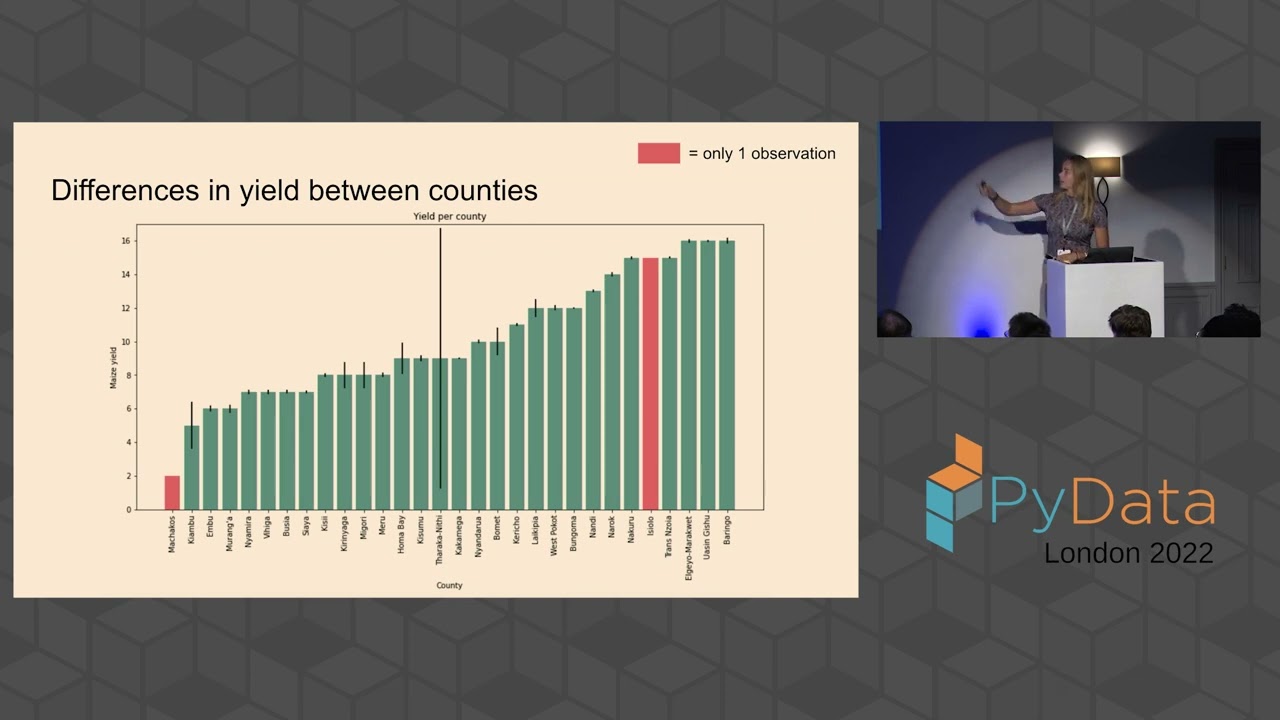
Bayesian Hierarchical (Multilevel) Modeling, which allows for sharing information across groups in structured datasets.
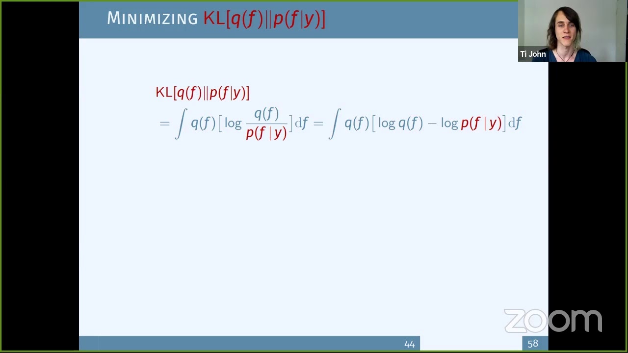
Variational Inference (VI) as an optimization-based alternative to MCMC for scaling Bayesian methods to high-dimensional, massive datasets.
Bayesian Machine Learning applications, such as Gaussian Processes and Bayesian Neural Networks for uncertainty quantification.
944 views9likes1:11:13Original Release: 2022-06-10
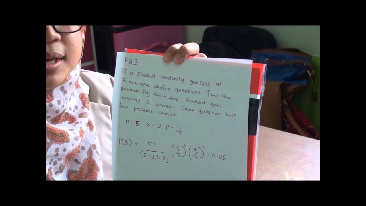
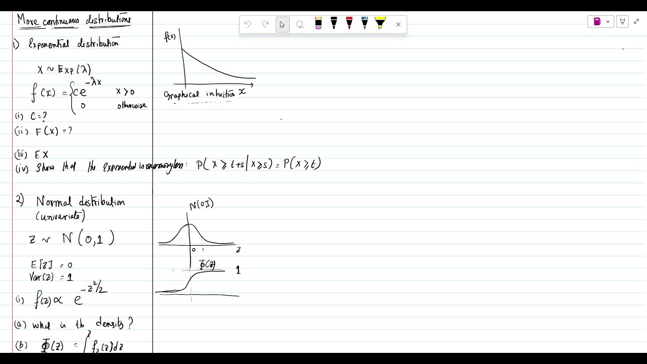
okay so these are some discrete distributions uh from which you should know these two by heart and this one maybe it's not that important so the binomial you can use it if you have like a maximum number and then you want to know how much from that number if the occurrence so uh that's k the occurrence of defense and the total number a piece of probability so this can be used for except for and 40 coin flips and then see how much uh head comes up and how much still stuff like that for everything that you have a maximum if you don't have a maximum you can use a poisson distribution that has a rate that you can use for uh for example uh car crashes because you don't know maximum car crashes but you know how much on average will happen and then you can use that is this that's the lumbar and then k is the number of occurrences that you will sample uh and the bernoulli is uh the special case of the binomial where you have one coin slip only or one n and then it will come to this because if you put an n here and one here will be one minus k if you have one double this it will be one so if you suggest uh you can use for one going flip or like this set parameters we saw earlier when you had multiple models and these are expectations they are not really important to know but maybe you can write them down if you want to is everybody done with writing or can i continue oh yeah boom okay so these are some continuous distributions uh you've seen the beta yeah if you've seen all of them btag is used as prior for uh bernoulli and binomial distributions you have a shape parameter and a rate parameter yeah then variable x what's the most often it's x is theta and then you can also we saw that there's one exercise i think you can write a and b as this and then you can also do the other way around and then you have more like mean and standard deviation around the mean uh which can be helpful if you want to interpret the beta distribution uh it's between zero and one uh so it's useful for beta and bernoulli then we have the gamma distribution it's pretty similar but a little bit different but the difference is that uh here the outcome can be above one so you can use it for a standard deviation for a gaussian distribution or for a poisson or exponential and you again have a shape and a rate parameter very similar uh and then you have the normal i think you already all know that one so you have a mean and standard deviation and it can be negative can be larger than one it can be everything [Music] how do i just stop sharing there you go i only play fifa 40.
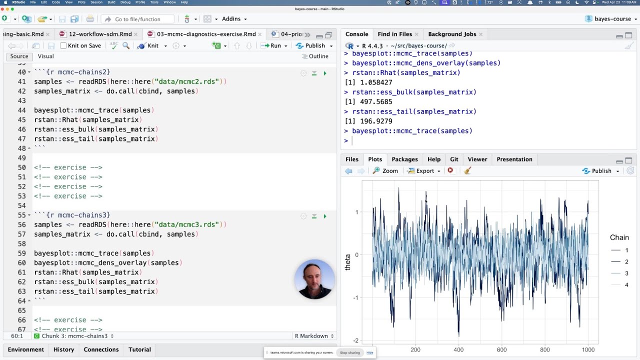
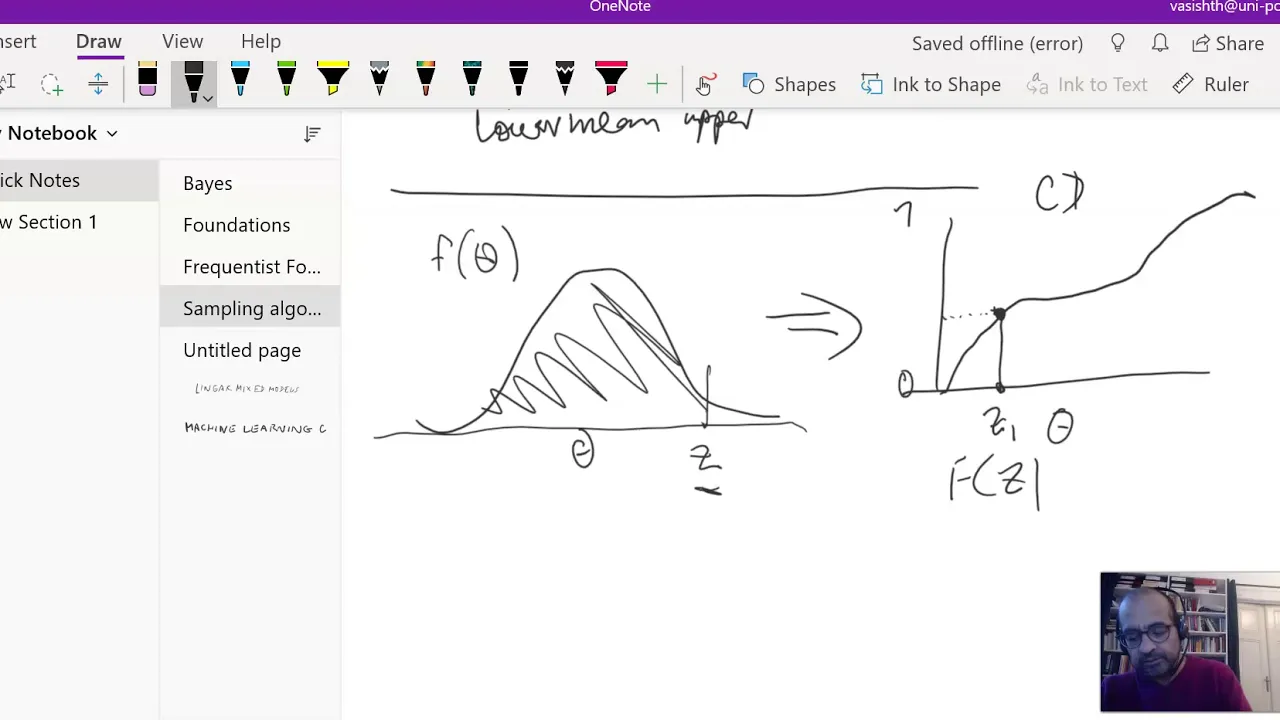
chicken head oh dragon hat yeah that's one yeah i think that's more precious than the dragonite yeah where is it oh my god should i straight from blue no position is this the one you were at yes okay gamma can be larger than one and b is between zero and one so therefore yeah yeah that's a bit i was also confused when i read it again my slides yeah yeah yeah but maybe i don't know this is this should be not bigger it should be larger than zero i think i was also good but you can use it for prior for poisson and uh exponential that can have numbers larger than uh one so i think it should be larger than one yeah so that's used for coin flips or stuff like that uh yes i didn't make this flight last year so maybe there are some mistakes in here i will put them here or i did make it did i just say i didn't make it yes this is the beta and this is gamma hello online this is the gamma distribution and this is the beta distribution so as you can see like oh maybe i should use this is a normalizing constant so that's why the beta distribution falls between zero and one this one doesn't have a normalizing constant okay this is the normalizing concept and this one doesn't have a normalizing cost it does have some division but it's not a normalizing constant okay what's that clear for online oh there are some chats yeah we don't even see the slides but that was five minutes ago so you fixed it right now we do great so the top one is gamma in the middle is beta indeed and the lower one is the normal that's correct no i think that's only for the beta uh yeah but there's a different you can also write a different note in this way but with a uh scale so this is shape and rate but for the gamma you can also write it as one over beta and that's the scale and then yeah it becomes a little bit different [Laughter] okay is everybody done and is there no more confusion okay let's continue yes so conjugate so i already mentioned some which distributions belong to other ones but the problem is when we do bayesian inference uh the marginal likelihood of an integral and it can be infinite or intractable uh so we can't find the posterior distribution so the solution is to use conjugate distributions so the posterior has the same form as the prior so if you use a beta it's prior for bernoulli that posterior will also be a beta between different parameters same for everyone on this list and the conjugate prior of normal distribution is just a normal distribution and to find the posterior you can use the proportionality so because the marginal likelihood is one number so if you divide it it doesn't change if you leave it out it doesn't change the shape of the distribution with only the scale so you can to find the posterior parameters you can also just multiply the prior with the likelihood and we will see an example that later yes can i continue okay so mcmc yeah monte carlo something something the basic idea is that you approximate the posterior by creating random votes through distribution according to some criterion so we know the likelihood and the prior priors often uh flat so we only look at the likelihood and then we propose samples and see if they are better or worse in their likelihood and if their posterior has more likely areas it will the random bug will visit those areas more often so how do you do mcmc you start at a random location and then you make a move to propose location with this and then we accept that move using this uh formula so we divide the proposed location by the current location and then if it's larger than one we use one as previously so it's we always go to the new location if it's lower than one so the current is better than the proposed then uh that's the probability and so there's still a chance that you go to worse the worst location but sometimes you also stay in your location uh yeah that's it is mcmc clear because i think you also work with it a lot so you know how it works and you don't have to apply it you only have to know stuff about it i hope for you so how do you check convergence so you can use mcmc because if you don't run it for enough iterations if the random walks are not similar and then we can make a good conclusion so you can use phrase plots similar and that means we can make a good this one you can see if burning is necessary so this one we can see at the start they are really different they become more similar so we can burn in different samples and auto correlation i don't know if it was in the lectures this year but it means if there is some some other variable that influences multiple variables then the samples are not real because they're based on each other yes oh yeah so that's because they're really different so we only take the samples from and that's why it's also important with multiple change because you can see if it has converse if you only have one chain you don't know if it does go first uh i think that's just my voice that the sound is weird uh what's wrong with the sound or are you do you know what's happening because it's in the chat oh it's fine now sometimes it cuts out okay whatever where is it okay so the most important part of base statistics is model comparison uh we want to uh so you can use this to get the parameters based on a given model so we can use base rule but we can also compare two models and see which one is better or more likely given the data so we have prior odds base vector and posterior odds and then if the base factor is higher than one model one is better and if it's lower than one model two is better but then depending on how big or how small it is and it's more it's better evidence and yeah so this only used one model and to get parameters given that model and this is to compare two models yes so more multi-comparison yeah if you this is what's on the last slide with this i think it's an example so if we have these two given set and n so it's a binomial distribution we can uh that we don't know the posterior distribution so we can calculate in this way uh most of the time we don't have any prior odds so both are zero to five and then if you divide them it's one so we only have to complete this part you shot up many times before and then here are the two the two models are these examples from the slide two models are this and then this is the data and we can calculate them using the binomial stuff and then we get these two outputs and then we can divide them because we have this so this is the base factor so we see model 2 is better than model one prior also this already mentioned that so the posterior this and using this magic we can calculate the posterior odds of the posterior probability for both models so we know that the sum of both models is one so we can say probability of model two is the same as one minus probability model one and then if we fill that in here you get this this divided by one minus model one is that number and then you can re arrange that to this then you can calculate that and then if we fill it in here we also get the posterior probability of model 2.
is that clear yes okay the savage digging density ratio you also work with it so i hope you still know what it is we have not two different models but we have two different hypotheses so one is zero hypotheses where for example difference difference is zero or weight and we want to see if it's important or not uh and then we can test these two so h1 is there is a difference or the weight has a value that's different from zero and then we can compute it this way so model one is hypothesis one model two is zero and yes no the other way around so this is for okay yeah no it's the same uh but this is for the prior this posterior so here we didn't see the data yet and here we did see the data so uh if uh the problem is higher than one it means that there's more uh probability or more evidence for that's the difference yeah here it's zero to five but let's say h zero so there's more uh evidence for no difference or a value of weight at zero uh in the prior so before we saw the data done after we saw the data so that means that probably h1 is true but if this number is smaller than one it means that there's more evidence in the posterior for hypothesis 0 so it means that hypothesis 0 is probably true because given data it's more likely that there's no difference is that clear okay uh some important basing concept so shrinkage i think you saw that one in practice in the practice extent the first question that you have three different settings and then with five data points and if we would combine them as one uh setting of 15 then we would it would be influenced by the prior by the outliers a lot and we would get mean this off if we use a generator model like this with shrinkage then we can say two are around this mean one is an outlier clause but it doesn't influence the or the omega as much is that clear what shrinkage does so you can have different parameters for every setting or every mobile yes yeah and it decreases the difference between variables they put them together because you have a prior uh okay then we have occam's razor uh that's like more just a statement among competing models the one with the fewest assumptions should be selected so if we have this one is more specific but less complain i read about it again okay so if we have two models one is very complex one is not complex and uh for example if the data is the very simple model doesn't perform well then we choose very complex one but if they both perform well so around this part can only explain a little bit of the data well this one can explain a lot of data but around this part we choose this model is that clear yeah so uh uh in the example exam we had three data sets or three settings and two had like convenience 9.8 and another one had a mean of six or something and if we would put them in one like we just calculate the average then it's very much influenced by the outliers but if we would put a like a prior on it and like this each setting samples something from that prior then that prior is less influenced by the outliers because it's it yeah it pulls everything together so it's uh it's less influenced by outliers and yeah it can estimate the mean better i think you if you do the did you already look at the practice exam i i think if you do that because i first also didn't really understand if you look at the first exercise it becomes pretty clear what i mean with it maybe you can look at it after this and i can still explain it if it's necessary okay where is my muse so more one more important basic concept the posterior predictive uh i think you saw that multiple times during the course uh when i did it it wasn't there so i have not experienced with it but you predict new data points given model trained in previous data we saw that with the game of thrones regression so we first train it on some data then we sample weights and then we get a new input and we calculate a new y if in those weights you can use the estimate but then you only get one weight or one value for each weight and then you only have one failure for y but if you use the posterior predictive you get samples from weights and then you can have like a distribution around y and it's more informative because you know the standard deviation and the uncertainty around that prediction why is that clear yes they still remembered from that exercise of game of regression not everybody completed that one no okay should but do you understand this okay now i have an exercise for you do we need a brake light or after this exercise okay but not yet or do you want to break okay so we have this likelihood in this prior binomial vita and uh i want you to write down the posterior distribution using the idea of proportionality which i mentioned during the conjugacy slide so you only need the posterior not the marginal likelihood everybody a favor i he's good stuff foreign yes together [Music] foreign [Music] does everybody know what to do or are you already finished should i give a hint uh yeah i first have to think of it so uh i think you all wrote down the distributions before right so you can fill them in and then see what performance and multiply them and then you can you have some stuff that's to the same like has the same base and you can multiply stuff and then base base coat [Music] so cute illusion okay you can just get the parameters foreign with her so did you calculate a did you multiplier the prior and the like i just speak a little louder everybody knows [Music] yeah okay but you brought that drop between them that's what i meant okay so yeah so i think your x should be a b or your b should be an x yeah do you now see what you can multiply oh um yeah the p and the x in the likelihood and prior that should be both be tita if you want to follow this with fi to usb or edge the clip yeah what do you get then uh [Music] what did you [Music] let's yeah okay the out the formulas and multiply them and they can rearrange terms that just stays there okay i will just explain it later what you can do okay i will continue i will show the answer step by step so we have this is the likelihood so x is k here it's a bit confusing and then this is the prior so we can if we would multiply this we can see we can have this with this and this or we can add the powers of theta and the powers of that and then this is the posterior uh yeah the formula for the posterior this is what is proportional to only a normalizing constant so the shape doesn't change and the power of theta won't change if you find it like this it will only influence this and this uh which will result in this because we added the powers of theta x plus alpha minus one and one minus theta which are n minus x plus beta beta minus one so we get that and now you can see it has form of a beta distribution again and we can fill in the parameters so if we look at the fryer if we use alpha as alpha we get alpha minus one here we have minus one so the new alpha is exponent alpha similar for the new beta so that just yes uh yeah that's also only a normalizing constant so uh if you say proportional it has the same shape but the skill can be different uh this only because there's no theta in here it doesn't influence how high everything will be if they should be here but then it won't fully match this we will see that later but this is like the most important part that's like the signature of uh the beta distribution right yes yes so this is also proportional uh because that's just how a beta distribution works so if we have theta given alpha beta they're missing here then we fill this in so it's alpha minus 1 here we have f the new alpha is x plus alpha okay then uh now that we know the posterior we can calculate the marginal likelihood uh i will just show this because why is the integral removed in the second step of the posterior because that's only a normalizing constant the result of that integral will be one number so it will only influence the height of the distribution but not influence the shape so we could say it's proportional to without the integral because the relative difference between two points will be will stay the same yes so okay these images are really poor uh can you still read it okay so uh now i change the location of the let's go of the posterior and the marginal likelihood so this is the marginal likelihood to know like the normalized constant this is not posterior because normal bayes rule is this over here and this over there we can just multiply both sides with this one and then divide both sides with this one and we now already know this one so we can use it to calculate this so to calculate the marginal likelihood uh with the parameters we found so x plus alpha and n minus x plus beta so those are the new alpha beta posterior distribution you can also fill them in in normalizing constants so now we have this is the full posterior distribution so first we only have everything this so first we had this but oh but now because we know the parameters of the posterior distribution we can also fill them in in the normalized constant this part and then you see it's similar to this one but with x plus alpha and n minus x plus beta so it's similar to this uh if we then yeah just rearrange stuff we can multiply this again this is what we saw earlier as the posterior we found or the uh proportional but now with n over x and one minus uh one divided by the beta distribution our beta function with alpha and beta and then if we divide you you can see this and this can you also see it okay um yeah this is just the the theta and the one minus theta and its power so this and this is the same uh and we can divide both sides so the result is this so we only have this part this part and this part and then we can rearrange it even more to this so this is the normalizing constant as you see there's no theta in it so that's why we can uh leave it out when we want to find the proportional posterior because it will only influence the yeah the height of the distribution do you see that yes yes so it's proportional to the likelihood of fryer the whole posterior is uh this part this is the posterior but we can say it's proportional to the shape is the same influence it stays the same on a different level uh without this integral but it's still similar right if we then want to calculate this we can multiply both sides with this so then we would get this times this is this and then we can divide both sides with this so we will get this this is that divided by this which we see here but with difference yeah it's written in a different way maybe can i draw on this on that one is [Music] so is that clear nice watch okay yeah then i open two exercises about generative and graphical modelling also with oh it's clear for everybody in the chat okay nice you can always re-watch it or re-watch the stuff from last year because there's another example in that one and just write yourself a different conjugate distributions maybe uh do you want a break right now and then we will do this too or do you want to continue yes okay then we will continue guys okay do this exercise so another farmer grows apples this is from when i did the course the practice exam so i didn't write it over the course of 30 years she knows that the apples in why i in year i or orca depends at least on the soil quality index that year xs i uh two the amount of sprayed fertilizer the year x f i so we have multiple x's and the number of injected pesticides that year xbi constructive patient model that the farmer can use to predict the apple yield for next year if uh yeah and then x i plus one that's a vector and are these three numbers so the next x you don't have to do much with this just contract constructivation network that should get example a y from x how you should start okay what is the output variable one yeah yes so uh what distribution can we use for or what kind of variables why is it between zero and one is discrete is it continuous can it be negative yes and not negative so okay a bit weird he still uses gaussian so it can be negative and not discrete so you can assume you can use a gaussian so we can use a gaussian to sample wise what should be the input gaussian which is the variables yeah uh what standard deviation what can we use yeah just something we said for each one or another variable that is a prior but you don't have to get any information from this for the standard deviation most sometimes you don't and what can we use as mean which variables are left in the text which we can potentially use yes so what kind of model is this yes so how do we want to use all these x's for a mean yes and how can we then construct such a b we have three x's and the outcome is one number so how can we combine those x's to one number no yeah or just add them you can also take the mean indeed but uh like we saw with the games of regression so we did multiplied each x with a weight and then added them so is it now clear how you can approach this because that's almost everything they still need a prior on your weight yes [Music] because often in regression models we have an input of the model for example with the coin with a coin flip you don't have an input you just have the sample output from distribution here we have an input of three axis and then uh we want to combine those to predict a wide so that's a regression level uh my okay okay so why was the outcome variable we could sample it from a gaussian so write that down yeah yeah yes that's indeed a little bit weird but that's what you did in the uh example maybe uh poisson would be better than and then with a raid that's also but yeah that would be that's not the only answer with a gaussian but i just want to follow his solution my solutions do not confuse you any further which for some would maybe be better yes so we have mean and standard deviation right just write a mu and sigma you can always later mu and sigma no that's a theta mu is the yeah but that's that's for mcu that's the location what is it [Music] does anyone need help or already finish it i'll give you one more minute so what do we usually do yeah so and how can we combine them yes yeah we don't multiply each x weight you can sample that weight again or as well from another gaussian yes or from something else but a gaussian makes more sense because then it can be negative for regression it makes sense that a weight can be negative because it can also have a negative correlation no one the mean is deterministic because we have three x's and three i would just show the next one i think everybody's done except for you yes so this is a generated model in a graphical model i will first explain the generated model so we said we start from the bottom down because that's easiest to understand it you sample y from a gaussian when it means sigma the sigma is yeah because uh yeah because in jax you always use one over sigma squared right as in the gaussian or you sample something from the gamma and use that as the standard deviation but the standard deviation inject is one over sigma so we have to infer the gamma if for normal but if you just use a gamma it's also fine what yeah okay so we sample uh the standard deviation from here it's not really important but you fill in you can also just use an a and b or something like that you don't have to write or define the hyperparameters and then we can define the mu as a weight zero so that's an intercept because we don't always want the regression to go through zero and then we multiply each of the three x's uh with a weight uh yeah and then we sample these weights from a gaussian with zero mean and one standard deviation we want to sample them from a gaussian because you want a way to that can be zero or that can be negative because it can be a negative correlation between two variables and you should not forget these and then grab commodore speaks for itself from the generated model so we have a y sigma because mu is not d or mu is deterministic it's not sampled but it's just defined you don't have to mention it in your graphical model but you are allowed to so the exit because this can also just be put in here doesn't make a difference for your model so you can leave a view but if it's easier for you you can edit yeah if you want the app here we would have a new that's also in this box so with i and then uh that one will receive these two that will go to mu u will go to y together with sigma okay yes because sigma is not a hyper parameter because it's sampled so it's not fixed it can change these are the hyper parameters of sigma but they're already defined and if they're defined you don't have to add them but if we would put an a and a b here or c and b w or if you would leave out this sampling and just have a sigma variable you can write as a hyperparameter i don't think it's necessary to have a square here because i think you didn't do that in previous exercise as well right you just write it down like that but if you can add it it's always better okay is it clear for everybody in the chat as well and here does everybody have any questions okay then i have another one that's the last exercise should i read it or can you read it at the back no i know you can read it or i i have my doubt uh so a group of ms-10 people are interested in investing in cryptocurrencies example given bitcoin you can see it's an old exercise they can choose to invest in any of 20 and it's 20 different of these currencies the probability that the person i invest in currency j depends on both the risk-taking nature of that person the i number between zero and one with zero is no risk and one is extreme risk that can be between zero and one so it's not a bernoulli as well as the perceived technical quality of the currency qj also a number between zero and one with zero's worse quality one's best quantity we observe only k i j which is one if i invested in j and zero otherwise we wish to learn both the risk taking nature of all people in the group as well as the perceived quality of the currencies yeah what model can we use yes your question it's a similar to the exercise we had in the second large assignment with the questions for students um so that doesn't do that everybody know how to approach this or should i give some hints okay so what is the outcome or to be predicted variable it's often also an observed variable so if k i j uh from what kind of distribution can we sample chi i j or what kind of values does k i uh j can have oh yes yes bernoulli what is the input of a bernoulli yeah one probability so how can we get that probability from this uh i think you're one step too far how can we make a probability from p and p and q are both probabilities well between zero and one no not really we have a probability that someone invests and we have probability of the or like we have a number that is the risk-taking so probability that someone uh takes the risk invests and we have probability that uh of that technical quality if we want to combine those to one probability yes you multiply them because if you find a number between zero one another a multiplier it will always between b between zero and one so that's also again deterministic so you don't sample anything you just say that probability is q p times q uh and then how can we sample b and q yes and why do we want to use beta yeah but there's also another reason yeah it's not really necessary for the general model but because the likelihood is bernoulli and because we often want to use a conjugate so if you use a uh poisson then the flyers often uh gamma if you use a beta or bernoulli the prior is often uh binomial or benue the prize conference and if you use the gaussian the price of the linguist as well except for the stigma that's often sampled from from a gamma yes yes you can do that but then you lose the conjugacy so if you want to apply that model in real life you can only do it once and then you have a very difficult model so you cannot incorporate more information so that's more it's not really necessary i don't think you will get any points of track but just for your future yes yeah yeah yeah that's the same as uniform it's it's a flat priority code so you don't have any information in your prior every probability is equal so we can use theta one one okay can i continue to show the answer yes okay so this is the answer so we already walked through it so you sample k i j from bernoulli theta i j don't forget the i j here because we want a different theta for every combination of a person another person yes i want to mention that later i will first explain this and then mention that so don't forget i j and then we can say that is these two multiplied we don't need this like a wave because it's not a distribution uh and also don't forget the ranges here and then we can sample both from a beta you can fill in one one or something else but make sure it's not too strong because you feel in 101 it's a bit weird that you fill that in without any reason or you can use alpha or an a and b but you don't have to define anything from them and then if we look at the graphical model uh we have the e and the q again this is deterministic so we don't have to include it but you can include it and then you would have here so this k should be uh between boxes as well one box for i one book because what he did yeah no it's not it's not wrong it's just not very quickly and you get one big box around everything which this one doesn't use i this one doesn't use j so you want to have different boxes yeah this should be this should be in both boxes these should be in one so you would have something like this so this is also incorrect because this one is not in a box for some reason yes [Music] but you can use capital or not it's neither to use capitals yes you can still do it but it's not necessary even if you have one one here you can leave them in because they would represent this one one but you can also say one one and pick them out is this one there this one was that was it for for the crash course but i can still answer some questions maybe about the practice exam but there's something difficult about that one is it difficult okay you're welcome [Music] no it's not most support for the exam but the most like for future for the exam i think you just have to know some concepts know how to do the math yeah you will get probably i don't know but i think in most exams there's a question about it right oh you didn't look at it yet but i think in most exams there is a question every question is about model comparison oh the next okay oh [Music] yes oh [Music]
Up Next

5:11
Beta Conjugate Prior to Binomial and Bernoulli Likelihoods
@oxeduc4209
49.7K views•2014-08-12

4:43
Elliptic Curve Cryptography Explained: ECC, ECDSA, ECDH
@PracticalNetworking
28.5K views•2024-10-21

10:44
Fourier Series Introduction: The Big Idea Explained
@DrTrefor
387K views•2021-05-03

6:00
The Mathematical Impossibility of Accurate World Maps
@Vox
23.3M views•2016-12-02
Related Study Plans & Knowledge Roadmaps
Structured learning paths in Mathematics
mathematics
Tensor Calculus: Vectors to Riemann Curvature
01Mathematical Foundations: Linear Algebra & Calculus
02Covectors, Dual Spaces, and Tensor Basics
03The Metric Tensor and Index Gymnastics
+ 2 more learning modules
40h5 modules
Explore Roadmap
mathematics
Gödel's Incompleteness: Logic, Proofs & Limits
01Introduction to Formal Systems & Hilbert's Dream
02Set Theory, Cardinality, and Cantor's Diagonal Argument
03Arithmetization and Gödel Numbering
+ 2 more learning modules
14h5 modules
Explore Roadmap
mathematics
Galois Theory: Fields, Groups & Solvability
01Foundations of Abstract Algebra: Groups & Fields
02Polynomials & Field Extensions
03Splitting Fields & Symmetries
+ 2 more learning modules
24h5 modules
Explore Roadmap
mathematics
Non-Euclidean Geometry: Models & Geodesics
01Euclid's Fifth Postulate and the Birth of New Geometries
02Hyperbolic Space and the Poincaré Disk Model
03Geodesics: Defining Straight Lines in Curved Spaces
+ 2 more learning modules
15h5 modules
Explore Roadmap