![[TP] 2. Metryki. Jak odległość określa topologię?](https://i.ytimg.com/vi/Pe6gDKKDOu4/maxresdefault.jpg)












![Why Does Persistent Homology Work in Applications? [Adam Onus]](https://i.ytimg.com/vi/x9ihVVV-bzc/maxresdefault.jpg)
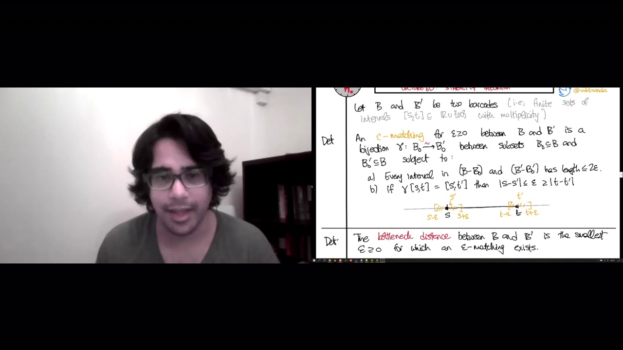

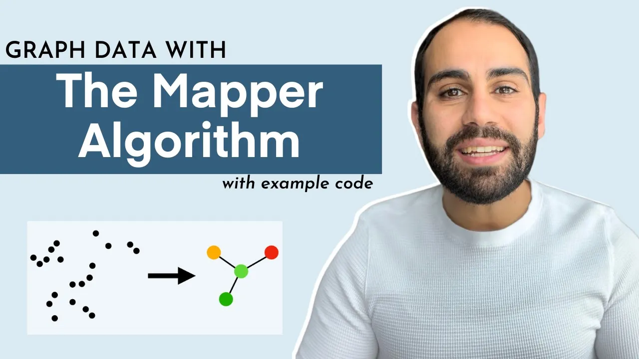








Topological Data Analysis (TDA) is a framework that extracts geometric summaries from complex data by analyzing the shape of data through functions called 'lenses,' which transform high-dimensional data into interpretable graphs that reveal patterns, clusters, and structures without requiring extensive statistical assumptions; this approach works by defining a metric on data points, applying functions to create inverse images, identifying connected components or clusters within those inverse images, and constructing a graph where nodes represent clusters and edges represent overlaps between them, allowing analysts to visualize and understand complex data structures such as identifying systematic errors in machine learning models or distinguishing between different classes in medical studies.
Topological Data Analysis for Big Data Applications
Added:all right all right thanks for for inviting me um so i'm gonna uh be talking about uh topological uh data analysis and um what my kind of meta message is that topological data analysis is a framework that integrates a lot of different machine learning uh data analysis and statistical techniques they sort of will live inside of the topological framework and by framework i don't just mean an abstract framework i mean it it's going to improve existing methods right like a good framework what it does is it doesn't just unify but it improves so i'm going to try and convince you of that for this talk and in particular i'm going to be talking about uh how how is the of use data and views data analysis uh one caveat is that tda itself is a bigger field than what i'm talking about here so if if you've heard words like persistent homology things like that i'm not going to be discussing them today i'm just going to be talking about the core algorithm that's being commercialized by ayasdi that's called mapper in the academic literature so what's our problem that we're addressing so we have um we want to extract meaning from complex data so data data is complex um for a variety of reasons one is that it's big data meaning it has volume and velocity however you want to phrase that but that's not the only way the data can be complex another way is it has very it can be very feature rich with a lot of complicated interdependencies between the features so there i'm thinking of let's say genetic data where for a given individual you can have 500 000 features if you're looking at snip data but there's complicated but your actual you know you you only have a small number of individuals so if you're thinking the individuals as rows and the features as columns you may have to say let's say a couple hundred rows and hundreds of thousands of columns and that's also a very complicated data set because of the rich feature structure and we want to be able to tackle both of these problems both of these issues so we want to be able to handle data that's complex because it's big in a classical sense but also just complex think about complex data so the way i think about complexity is sort of is in terms of a metaphor uh one that i like is imagine you walk into a room like a stadium and it's full of people talking right and you walk in and it just sounds like white noise and the problem is that there are so many different conversations happening at the same time and when you're tackling the data problem usually your goals are one of the following you either want to kind of zoom in on an individual conversation or you want to create a summary of the conversations of the in the room so in both cases you need to filter out the unwanted information another example of this kind of multi conversation structure leading to complexity would be looking at gene expression levels so let's say you want to study cancer and you study that by looking at how genes are expressing in cells and you have some measurement of of how sort of turned on the gene is or not um well you're interested in cancer but there's a lot of just regular cellular functioning that's happening in those gene expression levels so you want a way to just zoom in onto the relevant things that are going on with cancer while tuning out all of the irrelevant things so top tda topological data analysis is going to be a tool that provides summaries for us they're going to provide geometric summaries and so i'm using summaries in the kind of technical sense here topological data analysis will provide geometric summaries of our data so the central premise that we have at ayazdi is the data has shapen and shape has meaning and in this talk i'm gonna i'm gonna focus on the shape has meaning part which is how do we use the topology to summarize the shape and learn something extract some meaning from the data so before we start though maybe we should pause and think a little bit about shape so so one very compact way of saying what shape is is that it's the global realization of local constraints so there i'm thinking of something like a circle where uh you have a local constraint that's that bends the points a little bit right locally on the circle but the shape is when you step back and you see oh it all connects up into a circle so all of those local constraints in the data glued together in some global way to give the shape of the circle so how do we get a shape in the in the data problem well we first we have to choose what we're measuring about the system so we also call those features or again thinking of in terms of rows and columns these would be the columns in our data matrix and then we put a metric on the columns so that tells us what is the not on the columns the metric on the rows apologies it should say rows there so what we need to know is when should two data points be considered the same or if i relax that a little bit when should two data points be considered very similar so metric actually gives you a lot more structure than just that very simple notion but so for concreteness and for the sake of this talk you can always think about that i'm defining a metric uh on the rose but you should keep in mind and just keep it in the back of back of your mind and i'll come back to it a little bit later in the talk that that we can use more relaxed definitions of shape as well maybe you don't need a metric but just a similarity and in fact we can even relax all the way to just the topological viewpoint where all we need is an open cover of our data set if you don't know what that means don't worry about it we won't we won't use it so the goal again um just reiterating what i already said the goal of topological data analysis is to understand the shape without with as few preconceptions as possible so to provide a summary of the shape so if you think of a typical data problem that you might have you've gotten some data you have let's say rows and columns again if you want to use statistics invariably as soon as you invoke a statistical model you've already assumed a lot of things about your data that maybe you forgot that you're assuming one of those is that you've assumed some kind of metric structure usually euclidean on the data points and what we do in topological data analysis is we stop at that metric step in a certain sense meaning we don't make further statistical assumptions about the data we stop at the point where we've defined a notion of similarity and this is what i mean with as no preconceived is a bit of an exaggeration but we want to have as few preconceived notions of what's going on i and so like a few so without like a statistical model looking in the background because there's a lot additional assumptions beyond just just the metric structure that goes into defining that kind of model so once you've once you have a metric the data has a shape it sort of it occupies some volume of space there's proximity of various points to each other there's gaps there's holes there's flares there's bubbles there's all these things that are already in that very first step when you when you go to analyze the data you've already created and so we stop there and we say well what can we say now how can we summarize the shape what does the shape say about the data okay so the technique is actually very simple and i'm not going to need to show you any complicated mathematical formulas i'm going to be able to describe more or less exactly what we do just with pictures and i think that that actually speaks to uh the the profundity of the method and that it's not really complicated there are there aren't hundreds of terms that we're very carefully optimizing and balancing out against each other it's just pictures we're going to start here in in math world and that's just a conceptual place to start so i'm going to draw the data as a smooth manifold meaning i'm thinking of it not as discrete points but as just you know a sheet or or a sphere or a doughnut or something like that and when i say function you should think a smooth or a continuous function so what's a function function is just well it's a thing that i give it a point in the data set and it gives me a number i can actually relax those those definitions so i'm not going to need smoothness or continuity when we move into the data world but for the for the beginning here where we're starting off just think smooth or continuous to get the right picture in your mind and um and of course the data won't be on a smooth manifold and in fact we should emphasize that that in the real world when we look at data problems they're almost never the case that things are sampled from a smooth manifold so this is a mistake that i think a lot of people make when they move from linear methods to sort of curved linear methods there's an underlying assumption that the data is sampled from or sampled near some kind of manifold structure but if you look at you know you look at marketing data or you look at genetic data almost always sort of a more prototypical model is like big ball of fuzz with flares shooting off of it in various ways right it doesn't it's not really manifold the local constraints another way of saying that in a slightly more technical way is that the local constraints the dimensionality jumps around as you move around through the space you'll have areas where things fall along curves you'll have areas where they kind of fill out space so so even though i'm drawing a smooth manifold we don't need that assumption the method still works without it and uh we should just keep that in mind okay so here in mathworld uh this is my data so it looks like a pair of pants and i'm thinking of the surface of the pair of pants as being my data points that i'm interested in studying so i want to create now a geometric summary of this data space something to keep in mind as we create the summary is that although you can see the data here in reality because of the dimensionality that you're dealing with you can't directly visualize your data but you will be able to directly see the summaries right now i've drawn the data as low dimensional so you can see both the original data and the summary so you get some intuition of what the summary is doing to the data but in reality you have to remember you never have direct access to the data you can never see it directly so the input into this method is a function that i'm calling f and here the function is just mapping to the real line and i'm thinking of it as just mapping to the height function what i mean is that a point over here to find out its value you just go oh you just move straight to the right and that tells you the value of the function on that point can we get caught yes okay so here's the method and like i said it's very simple so i take a point in the image of the function p and i look at the inverse image set f inverse of p so all the inverse intersect set consists of all those points that go to p under this function and what i'm going to do is i take the connected components of the inverse image set and for every connected component or connected piece i'm going to draw a dot over on the far right so down here p there's just one piece this whole the circle is connected so there's just one piece in the connected component so i just draw one dot over here up here however if i look at the inverse image set that goes to q i have two pieces so that means i'm going to go when i draw a dot for every connected component of the inverse image i'm gonna get two dots and now i just sweep through all the values of this function with this procedure and i get this y this is my geometric summary so the letter y what have i summarized i've summarized that the pants have two legs in a trunk right but i forgot something too well i forgot the hole in the middle right so i've summarized the space one aspect of the space using a function so the summary is a summary with respect to a function so this might be more clear why why this is useful if we look at another function so now i'm going to take g as the function that goes down and this whole left hand of the pants goes down to this p prime so f inverse of p prime has just a single point which is on the far left moving slightly inward i look at the inverse image of a point q prime i get two sides of the pair of pants those two curves so then when i go down to write my g summary i draw two points and this continues and i get a circle in the middle section over r prime there's just one piece again so i get a line and then by symmetry on the other side i get a circle again so here i have a different function g that creates a different summary of the data this time i forgot that i have this y these legs and trunk feature what i remember is that i have two holes two legs so i get the pair of eyeglasses as the summary and this this is the method that we do like i said it's very simple we take data spaces complicated spaces and we create summaries and we're going to use the summaries to do things so here's a little exercise to make sure nobody's falling asleep so the question is what's the summary if i use both g and f at the same time so what do i mean by that i mean i take the product mapping g and f so the image is some region of the plane i take a point p in the in the domain i take the inverse image of p under this map i draw a point for every connected component of the inverse image of p so the question is when i do that procedure but this time using both functions what's the summary okay so i take this point p and i look at the inverse image under g and f the inverse images that is going to be the intersection of the two pieces corresponding to this to this direction in this direction g and f respectively which is just these two points so the inverse image of p consists of these two points so when i take the connected components of two points i just have two points again so what am i saying that the summary isn't a summary at all it recovers the original space that we started with so what's the point of that exercise it says that with a rich enough set of functions or lenses we can recover the original space we started with of course um this leaves us no better often it gives us some kind of psychological comfort that we can recover as much information as we want but it doesn't leave us actually better off because the whole purpose is to get rid of information because the problem is inherently too complex to understand but the idea is that we can choose a set of functions to tune into the signal that we want and we can forget or remember as much as the original complexity as we like so this is again what we do we take functions on the data sets we produce summaries modulus of details okay so why is this useful one way that we use this is it it gives us an easy way to understand how something we might be interested in is localized in the data set so here is an example we have supposed to be red i don't know does it look red to you yeah it's just oh it's just my angle anyway we have this red dot this red region in our data set maybe this is these are the patients that have a malignant kind of cancer maybe these are the people committing credit card fraud and we look at what happens in our summary they all end up in one little region of one branch of a leg so we might we were able to understand and learn about where in the data set something we're interested in is sitting well maybe there's two things we're interested in we have the blue region and the red region we have you know um two variants of cancer or something well there's a problem now with f they end up right on top of each other and we're unable to distinguish them but if we look using g we we can separate them out so different functions are going to be able to localize and inform us about different kinds of localization problems so this is kind of the way i've drawn this this is i would say an easy localization problem and by easy i mean the the data that's causing us problems or the data that we're interested in is in some kind of small isolated region in the original data set there are lots of classical methods that are going to be able to get at pulling out where that data is more interesting is when you have the set you're interested in itself has some geometric structure and is distributed in the data data set so this here is a sort of a more complicated problem that you're trying to solve the set of interest itself has lots of structure and the way i've drawn that here is just with this green green line that kind of that goes through a wide swath of the data set so under f it ends up getting smeared out across almost the whole summary so it's f is really maybe not as informative as we'd like because i look at my summary and i say where are the points that i'm interested in and the summary says almost everywhere so that's not quite so useful although i will say i have gained some incremental knowledge which is that it's not in one of those legs of the pants so even in these kind of bad lens bag you know bad lens bad function choice for the problem situations you frequently gain some incremental knowledge but you can see with g again g does a great job of localizing and tells me a lot about where the set of interest is in the data set so and and i apologize i i've switched from calling them functions to lenses and that's just because of the the product they're called lenses and then the academic literature they're called functions and they're called filter functions in fact and i sort of switched the terms around in my mind just because i have to use both of them in any case lenses inform us where to look in the space for some phenomena for easy localizations think the red splotch that we originally look at lots of different lenses are going to be informative and in fact you can make it a rigorous argument that almost any lens is going to for a nice compact region of you know when your points are in this kind of small compact region almost any lens is going to give you is going to tell you where they are in the space but for hard problems and by this i mean problems where the set itself has geometric structure or it's distributed throughout the data set we're going to have to be more careful about the lenses that we choose but even in that harder case we frequently from bad lenses still get incremental knowledge so i know it's not in that one of those legs of the pants right i learned that even though it's smeared out almost everywhere i do get something from it i've learned something okay so that was the math view by matthew i mean we were in the world of smooth manifolds um we didn't have discrete data points um and so now i want to show you how to move from this world of sort of mathematical niceties to the data world so the first thing we're going to do is uh we're going to fatten up the points so if i take a point in the image of a function so i have some portion of the real line most of those inverse image sets of the real line are going to be empty so what i do instead is i fatten up points to be open sets of the the range of the function so here i've drawn them as overlapping open sets u1 u2 u3 another way of saying that is that i take an open cover of the range of the function then i just do the same thing to those open sets what do i mean by that i mean i take the here i'm taking u1 i look at its inverse image set which is uh this area here right that's the inverse image of u2 goes from here to here and u3 goes from here up so i take all those inverse images i take the connected components of the inverse image and for every connected component i draw a a node so u1 u2 u3 good question yes when you um when you when you're working in the data world or something does the point if you if you find a point on the manifold and you project it down do you treat open set after you project when when do you so i start with an opening i start with the data set and a function i ca i would calculate for every point the value of that function and then i would create an open cover of you know the range of the real line between min and max okay right so that gives me doing this procedure gives me these four nodes or four dots and what i'm going to do is i'm going to draw an edge between two dots if their inverse images intersect so what do i mean by that well if you look at u1 and u2 there's this piece in the middle here where u1 intersects u2 so i draw an edge between the dot corresponding to u1 and the dot corresponding to u2 similarly up top on the the right there's this intersection here so i draw this edge and then for the other intersection here i draw another edge so instead of having a curve as my summary my summary is now a graph there's edges and nodes so what we've done this we've introduced some new parameters into the construction so i'm going to call the resolution the number of open sets in the range and the gain is the size of the overlap between open sets in the in the open cover so roughly speaking the resolution controls the number of nodes in the graph and the size of topological feature that we can pick out with the function and the game controls the number of edges or tightness of the of the graph that is produced as the summary so here what happens if i change the resolution so i've gone from three open sets to four open sets but if you just follow through what happens i end up with this summary it's actually very similar to the summary we just just had and that's because we're essentially already with three open sets at the maximal resolution we've already picked out all the topological features in the data set with just three so we don't really see a big difference by bumping up the resolution however we go down so i've gone down to just two open sets i lose some of the features of the data so i've lost the splitting of the pair of parents so i want to set the resolution to recover features of interest but setting it too high doesn't do me any good it just wastes space and and makes extra nodes in my graph okay so that's that's that now we need to do something else to bring this fully into the data world we still have the pair of pants where we're thinking of it as a kind of continuous sheet we need to move away from that so what i need to do is replace connected component of the inverse image with something i'm going to replace that with clusters so we're going to use clustering in the inverse image as a data driven way to define what connected component means we're going to connect so nodes now right i've replaced connected components with clusters so i'm going to connect clusters when the cluster share points in common so let's let's take a look at this here's my data space now where i've drawn a bunch of points instead of the pair of pants so i have this u1 set i do my i look at the inverse image it's that region of the space there i do my clustering on the inverse image i find i get two clusters and then i've drawn them over on the graph continuing on with u2 i do the same thing i get two more clusters but notice in the intersection between u1 and u2 there are some points they're going to go to some cluster when i cluster in u2 and they're going to go to some other cluster when i cluster in u1 and when that happens i'm going to draw edges between those clusters so here's an example of what that might look like now i just continue on through the data set doing this procedure the nodes are clusters and edges okay so we just continue on looking at all these open sets and doing our clustering and this might be what we get again it's a why the summary but it's more complicated because of the clustering because of the edge drawings but the basic fundamental thing that i've summarized in this direction which was that y shape i've retained by this procedure so that's it that's the whole that's the whole algorithm in the data world so key to this whole procedure are the lenses or the functions that we're using to create these summaries different functions remember told us different things about the data we had the eyeglasses and the y so to some degree this technique rests on our ability to find good functions functions to provide relevant summaries for the problems we want to solve and we're lucky lots of people have been working on finding functions on data sets so any kind of summary statistic on a row of data is a function on the data set so mean max variance and moments density s any kind of estimation of density is a function on the data set the function is what's the local density at the point that i'm looking at etc so geometry also provides a rich set of functions so centrality is something we use a lot we find it very useful that's measuring the distance from the center of mass of the data how far are you from the core of the data if you have if you are sampling from a manifold you can do something like curvature the local curvature there are other more topological lenses which here are harmonic cycles which look for circles or periodic behavior in the data set and we have a top sort of a topologically model-free way of finding those so machine learning also provides functions so unsupervised learning methods like pca or iso map mds disney all these are functions on the data so why is pca a function well if i've reduced to let's say two dimensions i have two coordinates for every point of the data set well i just say well that's two functions right each coordinate direction i call a function and then doing that embedding or that projection gives me two functions on the data set and i could use that as input into the system so this is what i meant when i said framework for machine learning all of these sort of traditional methods or a lot of them have created functions and the method just eats these functions and let me talk just briefly about this one here model error information so one of the big problems in in machine learning is um is overfitting another way of saying that is being able how do i distinguish between sporadic error and systematic error in my model the summaries actually give you a way to do that and allows you to tune your models to a much finer degree and i'm not going to have time to quite go into the detail but just i'll give you the idea and that's basically that the output is a graph okay and if you think of just for a moment think of the graph as being people who might potentially have some disease right and they're connected to each other in various ways and the question you want to ask is when is when am i at the start of an epidemic and when is you know do i just have some random cases of some disease and being able to distinguish between these two on the graph is the same thing as being able to distinguish between systematic and sporadic error so looking at the summaries we can see where in the model we have where in the data space are we do we have systematic error and where does it look like it's just sporadic now we can't necessarily identify all systematic errors because we could we can only check a finite number of functions but we can do a much better job tracking down and tuning out systematic error and machine learning models and then finally another source of lenses are lenses that come from the particular data problem that you study it so an example might be if you have patients in a medical study you can use age as a function or age as a lens or if you're looking at time series you could use dates as a lens as well so these are kind of data driven lenses that are specific to the problem you're looking at okay so i promised you something about insight and meaning from the data set while the functions do this for you as well they give you a way to interpret and to get a new sort of conceptual understanding of what's happening in your data set so here i'm thinking of the function as not being some random function but as something that has some intrinsic meaning to the problem you're looking at so an example of that would be gas let's say gaussian density or some other density measure here now i'm imagining my complex data i can't see it right before we were looking at it's a pair of pants now i'm saying you can't see what it is it's a black box it's inaccessible i have some function i've calculated this summary and i'm telling you that f is gaussian density it's a measure of density this summary if this is low density here and these are the high density region this summary tells me that my data is bimodal right so looking by knowing what the lens is i've learned something about my data i've extracted some meaning on the other hand if this the function i was using is centrality this says that and here this let's just say this here is like the close to the core the core of the data set and this is as i move away from the data center says i have two ways of being abnormal in the data set if the data set were was sort of uh uniformly in some blob in space this roughly says that it's elliptical slightly elliptical there are two regions that are going off from the core or maybe they have two flares going off of my data set so if f is the mean so i'm taking the mean of something in the row this says i have two groups of high mean data that the high mean data splits up in a basic way into two groups if this were error information from a model that says that i have two different kinds of error occurring in the data set so the units or the me or the um yeah the units on the lenses or the interpretation of the lenses allows us to learn from the summary about the data it's been distilled down into a simple story that then we can understand and incrementally learn more and more about our data in this way so another way to think about lenses is that they're a kind of geometric query on your data so your data you know it's it's out there it's formed by let's just say the metric and it's sitting out there and what a lens does is i kind of take the data i stretch it out along the lens and then i look at the slices right and i'm saying what's happening on all those slices and how do these slices relate to each other so i'm imagining here uh doing a heart disease study where i take a bunch of hearts and i measure a bunch of things about the heart the sizes of things and the volume and this and that right and i could take all those patients and just create a data space you know some big space of data where then let's say i could cluster just do clustering on that and that's just global clustering what does that tell tells me that tells me what different kinds of heart disease are there if instead i use age as a data lens what that says is how does heart disease differ as people age right it takes that same data set it stretches it out over the h line and because of the overlaps and the edges and stuff what you get is actually a continuous picture so without a lot of arbitrary cutoffs and biddings you get a continuous picture of how heart disease is varying as people age okay so that's the method and that's that's what we're doing i'm just going to tell you a little bit about some some generalizations that i didn't really go into at all so one is that we don't need a metric at all just a notion of similarity and in fact we're only using that to do our clustering so if we have some abstract or extreme external way of doing the clustering that's all we need so lenses they don't have to be continual continuous whatever that means for the data space but they should be sensible meaning you don't want to choose a random function as a lens lenses are most useful when they have meaning extrinsic to the problem that you're looking at that's not strictly speaking true that they have to have extrinsic meaning but they still have to be sensible so an example of something without extrinsic meeting would be say like an auto encoder something that you've fit to the data in some way it doesn't really have external meaning because it's fit to the particular problem but through a lot of experience you know people believe that these are sensible things and so auto encoders make fine lenses so sensible you know it's it's it's one of those terms it's like the supreme court right you know it when you see it we don't we don't have to get pedantic about what's sensible means the other is which we touched on in the exercise you can use multiple lenses at the same time even more importantly lenses themselves don't have to be real valued they can have values in other topological spaces all we really need is an ability to create a open cover of the image space so you can map to circles you can map to anything is that a good misconduct we could discuss missing data sort of is neither here nor there as far as as far as the method goes we can talk about what that what i mean by that afterwards right so here we have open covers so in fact all we do using the open cover on the image space is we use that via the function to induce an open cover on the original data space so if you have some way of making an open cover or a overlapping partition of the space um then you don't need the lens at all so the lens itself is not is not needed necessarily for the construction so what that means is that the input space doesn't have to be rows and columns it can be anything with the topology in particular if you're interested in graphs say social networks that makes a great input space for the method you just use there you can use the graph distance or if you want you can do some kind of embedded graph distance or you know there's lots of ways of assigning uh lengths to edges and all of those work and then finally that the output is not really just a graph if you follow through all the machinery and you do it carefully the output itself is itself a simplicial complex and it can contain higher simplicities than just the edges but that's also been completely swept under the rug so i just want to show you now some some examples of of what the output looks like so this here is an online fraud model from a a major retailer so they tracked a lot of variables about the customers how long did it take them to fill out credit card information how many cl you know clicks did they visit before they ended up in their shopping cart what browser are they using what's the browser string is javascript enabled etc etc right there's all this information about the customer and then what they want to know is is this transaction fraud or not so we created a space out of all that we actually used an auto encoder and i apologize i don't remember what the metric is right now and what i've done here is i've colored the the summary by the fraud score that was given to us by the online retailer so they created this you know they have their machine learning statistical experts who have created this fraud score and what you see here you get this kind of rainbow pattern that says on a very coarse level the the geometry agrees with this fraud score that they created using some other method completely we don't know what it is they never told us nevertheless we see that the geometry in this fraud store score our kind of course agreement to us and the way you see that is you get this nice continuous gradient of the fraud score across the two pieces now you notice one of the pieces is much higher fraud than the other one um there so what we can do is look at in that data set look at chargeback information so this chargeback information is a kind of ground truth in this problem so this is when someone calls the credit card company after the transaction has gone through and says hey guess what someone stole my credit card i didn't make those purchases on your website so what here we've done is we've looked in their network at where this chargeback information is occurring and you can see that there's this big red piece up here and this is what i mean by this is the signal of systematic error in their model meaning that something is systematically going on that they're getting a lot of chargebacks that they're missing up in that area of the data set so we were able to go in and look at what those um what was causing those and what we found was that they had a lot of time on the checkout page so they took a long time to fill out the page this was being skipped by the fraud model because most of the fraud is committed by bots who are very fast so they had missed this kind of slow fraud and they also had no flash and no javascript uh enabled and the story that that the um that the the online retailer told us is that they believe that this is what's called spousal fraud so this is where you use your spouse's credit card without them knowing about it and the so that's why it takes a long time to check out because it's a number you're not used to putting in and the lack of javascript um and flash made sense to them but not to me i i don't they were very happy with that i i don't understand why spouses would not have javascript enabled it doesn't matter the client said that makes perfect sense i don't know maybe old people with old browsers or something that they never installed flash i i don't know lady case that was the story they are we were able to track down the systematic error in their model that they had missed after spending a lot of time optimizing their model okay so here's how much i i don't see a how much time do i have that's fine am i okay all right um so i like this example here because when i first uh went to work at aosd i was talking with before i was hired well after i was hired before i started i was talking with one of the other data scientists there about a kaggle competition that had to do with smartphone data so he brought it up just as like a you know over lunch as like an item of conversation and um it's it's from the michael j fox foundation and what they've done is they gave out smartphones to people with parkinson's and people without parkinson's but they gave out a very small number of phones they gave out uh 25 phones right of which i think 17 were parkinson's and whatever else were the controls and then people carried these phones and if you know data from the phone sensor was recorded accelerometer information um there was information about the the voice spectrum of phone calls like the you know the like whatever they gave like these blocks of of four-year coefficients for the phone calls all this data and in fact so you had you had 25 people you had like terabytes of data per person everyone you know you think at first maybe you think oh yeah parkinson's people shake more it's going to be easy to look at the accelerometer but you have to remember that this data in people carry the phones in their pockets some people have them around their necks some people put them in their purses there's like it's a complete disaster right there's no it's just like and so i had looked at that you know independently of ayazdi and i decided this competition was a waste of time and i was talking with this data scientist tamir about this and he was kind of you know because he had already solved it and what you see here is the um the these are all of the controls in the data set and these are the people with parkinson's and we're actually we're splitting the parkinson's patients into two distinct groups so and this is based off of looking at the accelerometer information so uh anyway i think it's a nice story um i like it because i was personally surprised that you could do anything with the data given right this is a classic extremely complex data but kind of small data in a certain sense because there's only 25 individuals in the study nevertheless we're able to really get a very strong signal for who has parkinson's and who doesn't so that's i think um yeah well at the end so for that example you must have choose the right lenses so throughout your talk the trick of your model will work is how do you pick the right lenses the formula of your equation so am i correct yes the lenses are important so but there are a lot of general purpose lenses right ones like the ones that come from statistics in this case this lens here is uh to be up here it's um centrality so it's distance from the center of mass so one of these flares is probably the center of mass player and i apologize i don't know which one and the other the other two are some kind of anomalous that's most likely what we're seeing here but like i said we have to look at it um i didn't do the analysis i'm not sure so these kind of lenses the point is that something like centrality we find it useful over and over again so yes in theory there's this like huge universe of functions that we could use but in practicality there's like you know there's things that that you know from statistics from geometry from machine learning and when you get down to it and you write down these kinds of intrinsic lenses there aren't that many so you just you can just try them and you can see what happens so it's a you throughout the experience it's a try and error you can just try them right every data problem is is unique you can you know you can use the lens as a kind of query like i discussed in which case that's a kind of a geometrical framing right you create a geometric framework for understanding the problem you make your geometric query you see what happens right so that's like you've thought through the whole thing from beginning to end you just apply that and you see what happens so that's one thing that's what i do a lot i like to sort of i imagine geometrically what the solution is then i just do it right but if you let's say you're like well i don't know what lenses to pick well then i would say just try some and see what you find see what the data starts telling you and then you know go from there the software itself has if there are things that you're interested in um like here you're interested in a certain outcome being localized right you want to separate out parkinson's from not parkinson's you can tell the software that and it will search for lenses and and metrics that that will do that for you and return them to you and you can choose to use them or not you know depending on whether you find them meaningful so uh so can you create a a custom lens like so so is is is a lens corresponding to a computation model and um so it's or like so how how that that can work so you have to comply like these combination models to comply with the topological frameworks to sort of work in those topography or a lens is just a function right so any place you get functions you can use as a lens so there's no sort of topological assumption assumption it's up to you to decide what's sort of my criteria for what are good lenses are that they have to be sensible so it's up to you to define what some sensible is choosing random values is most certainly not sensible right but sort of anything that has an internal logic to it is sensible yes so i was kind of surprised because you expect that before the clustering algorithm is very difficult to get the clustering nice clustering and such high visual cases like this it would be very hard to have that could be an initial clustering when you choose metric clustering and only cases that's right so hard to find so deep sorry for interrupting uh the the important part though to remember is that so the clustering is a replacement for this idea of a connected component and we've done all this binning so slicing up of the space we don't actually care to some degree we don't care about the precision of those clusters it's the overall structure that we care about and we find we do a very good job of even in these kind of sparse kind of classically bad clustering situations when you do it over and over again on all these different slices and then you piece them together you get very sensible results so it doesn't matter if an individual slice has the wrong number of clusters in it what matters is that like these are connect these get connected these clusters versus you know these that don't and it does as you go through these this sort of bucketing procedure the slicing procedure um it's just not sensitive to those problems so you you're clustering after you chose the i think you're mustering the entire whole space no the clustering happens in the inverse image sense okay so after you pick after you pick the lines after you've picked the lens and after you've sliced up the space into these little chunks so this the clustering happens there and remember the goal is to create is actually not to sort of individually create like the right perfect clusters i mean it's great if you do but like the goal is is like how are they all connected to each other and that turns out to be sort of an easier problem that's less sensitive to the details of what's happened on that clustering level right it's getting that picture that why right getting that whole summary if some of these clusters are wrong you just don't care about it um and i think that that's actually that that's really a nice wrap up which is that so how how do i view this kind of geometric viewpoint in the world of data analysis so from my perspective you know statistics is the tool that everyone's using right and it's a standard tool and that's good and it should be used but it's like you have a set of screwdrivers and the geometry is a wrench right and you've been using your screwdrivers to really good luck to solve a lot of problems but there are some problems that are just the wrench is just gonna is the right tool so there are some problems that are phrased geometrically that you know there's a lot of i would say there's a lot of low-hanging fruit for this kind of geometric viewpoint right now meaning i can walk into almost any place where anyone's building a machine learning model i can walk in take the data and tell them something they didn't know because all they have are screwdrivers i'm like well i got my wrench here and you guys have a bolt right um so what should you do well i'm not saying that it's better i'm saying you should use all the tools and all the tools is you know considering both the geometry and the statistics of the problems you're trying to solve all right thank you
Up Next

Essential Math for Game Development: Vectors, Matrices, and Trigonometry
@doxy_ai
576 views•2025-08-02
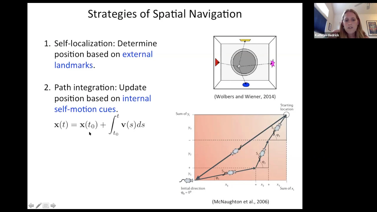
Gain Recalibration in Hippocampal Path Integration: Math Theory
@1024kyz
144 views•2020-07-02

Fourier Series Introduction: The Big Idea Explained
@DrTrefor
387K views•2021-05-03

The Mathematical Impossibility of Accurate World Maps
@Vox
23.3M views•2016-12-02
Related Study Plans & Knowledge Roadmaps
Structured learning paths in Mathematics