Essential Math for Game Development: Vectors, Matrices, and Trigonometry

[00:00:00]We're going to start by talking about space. Space is not the stuff outside the planet. So, it's not the stuff where all the stars and the moon and all the asteroids are. Instead, space is a line or a collection of lines. When there's only one line, we tend to label it as the x-axis. Then, when we have two lines, we tend to label the horizontal line as the x-axis. We've seen how what space looks like when it's a line. When space becomes two lines, it becomes a plane like this one right here. And even when space becomes three lines, it becomes kind of a a a cubical thing where humans exist. We also have higher dimensional spaces like 4D space and 5D space, but uh human brains aren't designed to understand those spaces visually. So let's look at some of the properties of our space. We've already identified that it will have an x- axis and that it will have a y ais and then in 3D space we also have the zaxis. The last one of relevance is the w axis. um why it goes X Y Z W AI has no idea the W should probably if we're being honest be like over here at the front but it might have something to do with what we're going to talk about in the next stream or two which is as a spoiler are called guians. So we've now seen the three uh the two or three labels for our lines in space. Well, we can start creating what are called vectors in the space. So, let's create this simple vector right here. You notice it has a couple of characteristics. It has a direction. It has a length and we can represent it by measuring how long it is along each of the axes. So, we see that it goes two along the x ais. So, we write down the two first. And we see that it goes another two along the y ais. So, we'll write down another two. This vector is slightly different than say this vector which if we notice similarly has the two along the x. So we can write down the same two but it has the slightly different y. It goes down a whole a full y four. So this is the vector 24. So we've identified what a vector looks like and we've identified how we can measure it. For any of the math nerds who are watching this retroactively, you might notice that I'm writing y backwards of how mathematicians would write it. Normally, y would go up instead of going down. That is an artifact of how monitors used to be designed. It used to be that an electron beam would go sweeping across the monitor. So it go from the top left all the way to the top right and then it would go down a row of pixels sweep across lighting some up. It would sweep across like that. So in computing graphics we usually consider the top left corner to be 0 0 where where both of the lines start and then x-axis increases to the right and the yaxis increases downwards the same way the electron beam of a CRT monitor would work. Why do we still keep that up?

[00:03:21]tradition. I guess it's not really necessary anymore, but shifting our focus back to vectors, we can do a couple of things with them. We mentioned briefly that they have a direction and they have a length. So, let's look into that a little bit more. So, let's go back to our friend 22. So, we'll write him 22. And how long is he? Well, we tend to write two arrows 22 to indicate the length of the vector. So, arrow arrow length. So, what is the length of our good friend 2? Well, to find that, we take the square root of x^2 + y^2.

[00:03:57]And in higher dimensions, it just scales. We add an a uh a z 2 and then we add a w ^2 and so on inside the square root. So in our case here, the square root of 2, sorry, 2^ 2 is 4 + 2 2 is 4.

[00:04:15]The square root of that is the square root of 8 which is approximately equal to 2.82 observation that number is a bit bigger than two. So the fact that a horizontal vector is longer than its sides is going to sorry a diagonal vector is longer than its sides is going to come up again momentarily. Well, what else can we do with a vector? So let's keep our friend 22 in mind. So our good buddy 2. And what can we do with him? Well, what happens if we multiply 22 by two? Well, what we wind up doing is we take the two and we multiply it into each element of the vector. All three in 3D, all four in 40, and so on. So what's 2 * 2? It's four. What's 2 * 2? It's four. So this gives us the new vector for four, which if we notice is very similar to our good buddy 2. He's just a bit longer. What can we do with a 22? We can wear it and we can multiply it by two. So if we start scaling vectors, right? What happens if instead of multiplying by two, we divide 2 two by its length? So we have 22. And what happens if we divide it by the<unk> of 8? Well, this it turns out will be equal to approximately 7.7.

[00:05:42]Let's highlight him in orange and let's draw him up here. So, it turns out that 7.7 is kind of a special boy. He has an interesting property. His length, so the length of 7.7 is equal to 1. Um, we call these special vectors with a length of one either normal vectors or direction vectors or unit vectors. That's the other one.

[00:06:11]Because they're useful for telling us the direction of something. If we multiply our little boy here by some number, so we scale them up to be longer, we wind up with a vector of that length pointing in that direction. Hence the name direction vectors. We'll also see them talked about in a little bit a little bit later when we talk about normals and that'll bring up the normal vector length. And then they're also called unit vectors cuz their length is one unit. So we've seen how we can scale a vector. We've seen how we can modify the length of the vector. What happens if we have more than one vector? So we're going to drop down two boys. We're going to drop down 1 3 and we're going to drop down 3 1. We have the vectors 3 1 and 1 3. So what can we do with them?

[00:06:59]Well, an immediate observation is that we can add them. If we're doing this component-wise, what does that look?

[00:07:04]Well, we just go straight down and add the numbers. What's 3 + 1? 4. What's 1 + 3? 4. So, this gives us the new vector 4. Follow-up observation. How does 44 relate to the other two vectors? Well, if we take our little blue vector and we move him to the tip of the red vector, it turns out that he will look something like this. And if we take our little red vector and move him to the tip of the little blue vector, he will look something like this. So, when we add these two vectors, we wind up creating this tilted square thing, what we call a parallelogram. and we're going to stick a pin in this idea of a parallelogram because they will become important later on. So just just keep that one in the back of your noggin. So let's drop down our two vectors again. It would be nice if we could find some vector that goes between them, right? Well, let's look at what happens when we do some subtraction. So let's write down the vector 3 1 and the vector 1 3. What happens if we subtract them? Well, just like addition, we go elementwise. So it's 3 - 1. It is 2. And what's 1 - 3?

[00:08:17]It is -2. Well, what's special about this vector? Well, if we look at it, it should go out a little bit and up a little bit. So, it should be something like, right? Well, what happens when we draw that vector at the tip of our two vectors? So, we'll draw it here. And there's not really anything interesting to observe about it there. How about if we draw it here?

[00:08:40]Isn't that interesting? So it turns out that subtraction finds the vector from second to first. So we wrote our vectors like this, right? Where we were subtracting the red one from the blue one. So we found the vector from the red one to the blue one. If we did it the other way around, so we did 1 3 minus 3 1, we would instead find -2 2, which is the same vector. And let's let's highlight it in orange, but going the opposite way when drawn at the tip of the blue vector. We have the vector going from the blue vector from the second to the red vector to the first.

[00:09:23]So how can this be useful? Well, let's take this vector uh 2 -2 and what happens if we find its length that will wind up being 2^2 + -2^2 of that equals the<unk> of 8 which we already identified was about 2.2. And then if we find the unit vector associated with this vector that'll give us 7.7.

[00:09:54]So we now have a short vector that points in the direction of this. So we can scale it and and find some vector of that length. The other interesting thing is the length itself is the distance between these two points. So if instead of viewing these things as arrows, we just view them as points in space. The length of the green vector represents how far away those two points in space are. Pretty useful information to have maybe. So, we're now going to do a small experiment. We're going to shift our focus a little bit over to 3D space.

[00:10:28]We're going to talk about something we can only do with 3D vectors. There are technically some versions of this that work in other spaces, but we tend to to really only think about it in 3D space.

[00:10:42]And that is called a cross productd. So to introduce a cross productduct, let's first introduce how we might define a plane. A plane is just three points or two vectors. So let's define the vector uh 1 2 and let's define the vector 21.

[00:11:01]You notice that these vectors have 1 2 3 points in space. And if we draw the plane represented by those three points, so it winds up being this flat plane on the bottom, we can make more interesting planes with points in in more interesting places. But three points or two vectors is what we need to define a plane. So given these two vectors, how might we find the vector going straight up? Well, how is this uh how is this useful? So say I want to bounce a ball.

[00:11:35]So, we're going to draw the 2D version of this. So, I have a ball and it's coming in towards the ground. Well, what direction do I want the ball to bounce?

[00:11:44]It turns out that if we take what's called the normal vector, the vector that's perpendicular to the surface, the the angle between the incoming vector and the outgoing vector should be exactly the same. So this angle and that angle should be the same. Talk about angles a little bit more in a second.

[00:12:08]But how can we find this perpendicular vector? Well, it has a rather simple formula. So the formula is x is going to be equal to the first vector which we're going to call a it's y and the second vector which we're going to call b its z minus the first vectors z times the second vector's y.

[00:12:38]Then y is equal to the first vector z * the second vectors x minus the first vectors x * the second vector z.

[00:12:50]We're getting a little bit of a pattern here, right? You notice how these are kind of the same form where we have the thing that's missing of the first two multiplied together and then we kind of swap the order of the thing, subtract it. Now the same thing here. The thing that's missing, multiply the two and then we kind of swap the order of it. So let's see if it holds for Z, which is equal to the first vectors X time the second vectors Y minus the first vectors Y * the second vectors X. So what is that in our case? Well, we said that this red vector was the vector let's do red 2 1 and this blue vector is the vector 1 2 and both of their third components both of their z's are zero.

[00:13:39]So let's put those in. So we have for x that's 1 from red * 0 from blue minus uh 0 from red time uh y two from blue. Then for Y, we're going to have the Z. So zero from red and the Y, so two from blue, minus, we're going to have the X, so one from red, and then the Z, so zero from blue. And then for the last component, we're going to have the x from red, which is two, times the y from b, which is two, minus the y from a the y from red, which is 1, times the y from b, which is sorry, the x from b, which is 1. So we multiply this together we get 0 - 0 = 0 0 - 0 = 0 4 - 1 = 3. So this vector pointing straight up turns out is the vector 0 03 and just like we wanted it happens to be pointing straight up which is perpendicular to the flat bottom plane. Turns out that the the length of this vector has a bit of an interesting property which we'll talk about over in 2D space. And let's draw that parallelogram that we saw earlier. So boop and boop. And it turns out that the length of that last vector, so the length of 0 03 of this vector is equal to the area of this parallelogram. So this has an area of three. Get rid of that little little line that looks like a minus in there.

[00:15:36]And get rid of this one, too, while we're at it. So what can we do with that information? Well, it turns out that half of the area of that parallelogram is the area of the triangle. So half the length of the crossroduct is the area of the triangle defined by the two vectors.

[00:15:59]It turns out that in computer graphics, a lot of the computations we do involve rendering triangles. And if we want to weight something by how big a triangle is, we can take its cross productd and then figure out how big it is from that cross productd and use that to weight.

[00:16:16]Very useful stuff. Um so last thing that it would be good to mention about the crossroduct is what it looks like when we write it out. So the crossroduct of 2 1 cross with 1 2 is equal to 0 03. And for this to be technically correct, we should throw the zeros back on there.

[00:16:40]Okay, so we've seen the cross productd.

[00:16:42]It turns out that there's another useful product with vectors. So let's clean things up a little bit. And let's start with a motivating example. So let's say that we have this vector and then we have this vector. Are they pointing in the same direction? And then we have this vector. How do all of these vectors compare? Well, so let's look at the blue one and the green one real fast. Let's write down what green is. Green is 31 and the blue is the vector 2 4. So if we take the dotproduct of this, what do we do? Well, we take their elements and we multiply them together element wise. So what is 3 * 2? That would be six. And what is 1 * 4? That would be four. and we add them up to wind up with a with the number 10. So what the heck does this 10 mean? Well, this 10 is a measure of how much these two vectors are pointing in the same direction. If two vectors happen to be pointing perfectly perpendicular to each other, the dotproduct of the blue vector dotted with the red vector will equal zero. So if they're pointing perfectly perpendicular to each other, so if they are normal vectors of each other, the dotproduct is zero. And if they happen to be pointing in approximately opposite directions, so say this vector, we have the blue vector dotted with orange vector and that should give us a number that is less than zero. So how is this useful? How do we interpret that 10?

[00:18:24]Well, let's tweak one of these vectors a little bit. Let's instead of talking about the full vectors, instead talk about one of them being a a normal vector. So let's drop down the longer one. So we'll pick that as the normal vector. So what is the normal vector?

[00:18:43]Sorry, the unit vector that we get from 24. The length of this vector is 2^ 2 + 4 2<unk> of that. So that would be 4 + 16 is 20. So the square root of 20 and the square<unk> 20 is approximately 4.47.

[00:19:06]So when we take this vector 24 / it by 4.47 we get the vector44.89.

[00:19:16]So we get the vector44.89.

[00:19:20]And then if we take the dotproduct of the other vector. So 3 1 with this. So we take 3 *44 which is equal to about 1.32 add it to 1 to the 89 and we get about 2.21.

[00:19:43]And what does this 2.21 tell us? Well, if we multiply 2.21 by the orange normal vector is the orange unit vector. So, if we multiply 2.21 by the orange unit vector, what happens if we make it 2.21 times longer? It turns out that that vector is what you get when you project the green vector onto the blue vector.

[00:20:12]So the dotproduct of a vector and a normal vector represents the length of that vector in the direction of the the unit vector. Okay, so we can use a a dot productduct to project a vector onto another one. Um how is this useful?

[00:20:30]Well, what happens if we want to calculate the reflection that we talked about with the cross product? So let's clear the screen and let's say that we have our surface. We have our ball moving in towards the surface. We know the normal of our surface and we want to find this blue vector. How can we go about doing that? Well, what can we observe about these vectors? The part that is going along the normal, right, is flipped. So if we look at this part, the part along the normal, it's the same, but this one's going down while this one's going up. Then if we look at the part that's opposite the normal, so normal to the normal or just the surface, you'll notice that these two parts are the same. So to find this bounce vector, if we can decompose the two vector the vector into a normal vector and a normal perpendicular vector, that'll tell us what the bounce is, right? So how can we break it down into those two vectors? Well, for starters, we want to find the green vector, right? Projected onto the red vector. How do we do that? We take the dotproduct of green with red assuming that the red vector is a normal vector.

[00:21:49]So assuming red is unit and then we can multiply that result by the red vector.

[00:21:58]Okay, so we're going to call this the orange vector. And then how do we find the purple vector? Well, the purple vector, the one that goes along with the that goes along the surface. So normal to the normal vector is just what's left over. So it's equal to the green vector minus the orange vector. And then the blue vector is equal to the negative the orange vector cuz remember we mentioned that it flips. So orange plus the purple vector. So what does all of that look like written out in in letters instead of just colored vector. So let's hide our 2D space to give us a little bit more room. So if we call the green vector uh d so the direction that we want to move in and we call our red vector n with a little hat. We use that little hat to indicate that it's a normal vector to to indicate that it's a unit vector and we multiply this result by our normal unit vector. That should give us the normal part. Then if we want to find the non-normal part, we take our direction vector and subtract that. So we subtract off d dotted with the normal vector times the normal vector. Well, we mentioned that for the blue vector, we want it to be the negative direction along the normal. So we want to negate this. And if we add these two together, we get d min - 2 * d n in the direction of n. Sound good? And it turns out that this formula is how to calculate a bounce. And it involves projecting our incoming direction onto the normal direction and then doing a little bit more processing with it. Make sense? So, it's now time to move on from talking about vectors for a moment, and we're going to start talking about angles. So, what is an angle? Well, we've seen that a unit vector falls along a circle with distance one from the origin. So, this is a unit vector. This is a unit vector.

[00:24:20]This is a unit vector. And we're going to talk about this blue unit vector in particular for a moment. Most people get taught in school that you can have three 360° to go all the way around a circle, which would then imply that you can have 180° to go halfway around a circle. That means that this blue vector is at both 0 degrees and at 360° since it wraps around. How about the black vector?

[00:24:53]Well, the black vector is about halfway up, so it would have an angle of about 45°.

[00:25:00]How about this red vector? Well, it's about halfway down, so it would have a ve of an angle of about - 45° or adding 360 to that about 270°.

[00:25:11]So, we can measure vectors based on their direction and mapping that direction onto the unit circle and then figuring out what angle you would need to rotate around the unit circle to get that vector. So, we just brought up rotations.

[00:25:29]How can we figure out how much we'd like to rotate the red vector to become the black vector? Well, we have to move 45° and another 45°. So, it's a 90° rotation. Cool. So, we've seen what a 90° rotation looks like, but how do we get it? Well, to answer that question, we're going to have to take a step back and talk about radians briefly. So, we mentioned that when you go all the way around the circle, that's 360°.

[00:25:58]And that when we go halfway around the circle, that's 180°. Well, it turns out that if you take the radius of the circle and you compare it to the circumference of the circle, so the big red line that goes all the way around, their difference is about 3.14 times. So the circumference is 3.14 times bigger.

[00:26:18]And this special number is called pi. We have a whole day dedicated to it. March 14th.

[00:26:26]March 14th. So how is this important?

[00:26:29]Well, cuz most of the mathematical measurements don't like degrees. They prefer a measure called radians. And And that then means that up here 90° is equal to p<unk> over4 radians. Just a fun thing to keep in mind when we start talking about how we do rotations. So how do we do rotations? So it's now time to bring up some scary thing called a matrix. So if we take this weird box with cos of angle negative sign of angle s of angle co of angle and we multiply it by some vector x y which we're going to write horizontally now vertically now this gives us a rotation. But hold up hold up hold up what the heck are these s and coine things? Well, it turns out that they're functions that have been defined in math. Sign measures how far up we are. So, if we go around, right, we're up zero and then at pi over4, we're up at 1. And then at 1, we're back down at z at pi / 2, we're back down at neg at zero. And then at another pi over4, another pi over two, we're down at negative 1. And then we're back at zero.

[00:28:06]So let's draw it out. So down here we're at zero. And then up at pi / 2 we're at one. Then down at pi we're at zero. Then over at another pi / 2 we're down at 1.

[00:28:21]And then at 2 pi we're back up at zero.

[00:28:24]And it winds up creating this sine wave type look. So this is s. Now let's see what happens with cosine. Cosine is measuring the x. So here x is 1. Then we go up to pi over 2 and x becomes zero.

[00:28:40]And then we go over to pi and x becomes 1. And then we go over another pi / 2 and x becomes zero. And then we go back to pi 2 pi and x becomes one again. So we get almost a mirror image this little slide. So at zero, we're up at one. And then at pi / 2, we've come sliding down.

[00:29:06]And then at pi, we're down at the bottom. And then at another pi / 2, we're back at zero. And then at 2 pi, we're back up at one. So it creates a very similar image to sign, just shift it over a little bit. And it turns out that if we have a vector and we know what its angle is, then its x component is going to be equal to the coine of the angle and its y component is going to be equal to the sign of the angle. How is that for a super brief no scuff at all introduction to trigonometry as fast as possible? So shifting back to our rotation matrix which we'll quickly redraw. Well shifting back to the idea of matrices. Let's not start with the rotation matrix. Let's start with a simpler matrix. So we're going to take the matrix 1 0 0 1 and then we're going to multiply it by the vector 2. Just remember that this is another way of writing 2 2 like we've seen before. So we have x and y. And of course these can get bigger. Well, what happens? We take a row and we multiply it by the col by the vector and that gets us the top of the vector. Then we take another row, multiply it by the vector and that gets us another slot in a new vector. So what does this look like in numbers? Well, it's like a dot productduct. So we dotproduct 1 0 with 2 1. So red please.

[00:30:48]1 0 dotproduct with 22. And then we do the other way. So we dotproduct 01 dotproduct with 2. And what does this give us? Well, when we work it out, this should give us 1 * 2 is 2 + 0. And 0 * 2 is 0 + 2. So this should give us the vector 2. Wait a second. Nothing changed. It turns out that this matrix where we have ones running along the diagonal and zeros everywhere else is called the identity matrix. When you multiply this process we just did the identity matrix by a vector, the vector doesn't change. So how about a more complicated matrix? How about we take our identity matrix and we multiply it by some some number at every element. So say three. So the one here becomes a three. The zero stays a zero. The zero stays a zero and the one becomes a three. Now what happens when we multiply it by our vector by our vector 2 2.

[00:31:52]Well, let's work out the dot product. We have 3 0 dotted with 2 and we have 03 dotted with 2. And what does this equal?

[00:32:04]3 * 2 is 6. 0 * 2 is 0. 0 * 2 is 0. 3 * 2 is 6. So this is wound up scaling our vector. So this special type of vector where the diagonals are sold some number greater than 01 is called a scale vector. So we already saw another special type of vector the rotation vector where we have cosine of an angle sign of an angle s of an angle and cosine of an angle. So what does this look like in an example? So let's say that we want to rotate by 45°.

[00:32:43]Well, it turns out that 45° is pi / 2. So a is p<unk> / 2.

[00:32:50]Unfortunately, when we're dealing with s and cosine, their input has to be in radians. So let's write this down. Let's write down cosine of p<unk> / 2 45° is p<unk> / 4 of p<unk> / 4 s of p<unk> over 4 sin of p<unk> over4 cossine of p<unk> over 4 and this is going to get multiplied by our favorite vector 2. So what are the numbers here? Let's go back up here. So about.7 about.7 about.7 and then about.7 we have our vector 2 two and then what does this equal? Well let's do the dot product. We have 7.7 dotted with 22. Then we have 7.7 dotted with 22. And what is the final result here? Well, 7 * 2 +.7 * 2 gets us 0 and the positive version gets us 2.8. And that kind of makes sense. If we go back and look at 2D space, if we have our good friend 22 here, and we want to rotate him by 45 degrees, which is this way since we're in sort of an upside down space, he should wind up landing at about 2.8, which looks like about the same length vector, rotated 45°. Make sense? So, we've gotten through quite a few things.

[00:34:29]Um, one more thing worth talking about while we're on the subject of vectors is what happens if we multiply two vectors by each other or two matrices by each other. So we have A B C D and then we're going to have E F G H. So we now treat the second matricy as two vectors. So we pretend that this isn't here and instead we have the vector EG and we have the vector FH. Well, we know how to multiply a matrix by a vector, right? We take the row, we multiply it by the vector. We take the column, we multiply it by the vector, and then we do it again. We take the row, we multiply it by the vector.

[00:35:17]We take the row and we multiply it by the vector. So we wind up dotproducting every row with every column. So what does this look like? Well, we get a new vector as the result, which is the dotproduct of AB with EG. And then we have the dotproduct of AB with FH. And then we have CD with EG. And then we have CD with FH. I'm not going to do an example of working this all out because it's a lot of tedious repetitive math.

[00:35:55]Um, and you just have a computer calculate it for you. That's that's the real thing here, right? Just let computer calculate. Your life will be much easier. Um, in a future video, we're going to talk briefly about some computer libraries to do these sorts of computations and and how they would work. But we've talked about 2D, right?

[00:36:17]Everything we've talked about with matrices scales to 3D. We just go row column row column. Same thing, but um and identity matrices work the same.

[00:36:26]Let's actually write out the 3D identity matrix, which is the matrix 1 0 0 1 0 0 1. Remember, it's ones all along the diagonal. Um but the rotation matrix is a lot more complicated. we wind up with a rotation matrix in like each of the corners. And it becomes a little bit weird to think about rotations as just a number, right? So if I say I want to rotate 45°, what does that mean? How do I rotate?

[00:37:02]Does a rotation of 45° mean a rotation around this axis or a rotation around this axis or a rotation around this axis or a rotation around some other random arbitrary axis? So, we start needing to think about rotations as an axis plus an angle. Um, again, I'm not going to work an example of this.

[00:37:28]There's libraries that create the matrices to do these rotations. Just use one of those. Life will be easier. Um, but say I want to rotate around some really weird axis, right? It becomes a little bit difficult to figure out what axis some arbitrary rotation should be around. So instead, we often use what are called oiler angles. And fun fact, Oiler is AI's great great great great great great great I believe grand adviser AI's was grand advisor somewhere was Alonzo Church and then up to Lelass and Lrange and then up to Oiler. But Oiler defined rotations as a rotation around the x-axis, a rotation around the y- axis followed by a rotation around the z-axis. How do we get this? We build the matrix for the y- ais. So matrix. Then we multiply it by the matrix for the y- ais. And then we build the matrix for the z-axis. And then we multiply it by that. We do a whole bunch of matrix multiplications.

[00:38:37]And we get a matrix for this rotation around these axes in this order. It doesn't necessarily have to be this this order. Some people give you ability to change the order. First you might do a zx y oiler axis but normally you think about them in the same order as space.

[00:38:54]So xyz. So there's a problem with these.

[00:38:57]When one of the axes becomes 90° you lose the other two axes start rotating around the same thing. There is at least one axis where that's the case. So if we draw an example, so we have a rotation around X and then we have a rotation around Y and then we have a rotation around Z. When Y is rotated properly, the Z and the X may lie in the same plane. This doesn't really cause any problems when we're trying to enter numbers. So, no issue for rotation entry, but there is a bit of an issue when we're trying to do like animations and blend multiple rotations together.

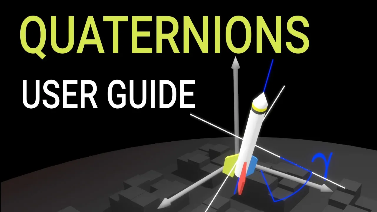
[00:39:42]So, I'm going to give a brief spoiler about the next stream where we're going to talk about the solution to this, which are a concept called quatronians.

[00:39:52]Um, so the last thing to talk about today is another type of matrix. So we've seen how to write a scale matrix.

[00:40:02]So scale scale scale with extra zeros.

[00:40:05]We've seen how to create rotation matrices. But how do we do a movement a a sliding a translation matrix? Well, it turns out to do that we need to go to 40 space. Just like a quatnian which we'll talk about next time is a 40 extension of rotations to make their their smoothing work in order to do translation we need to go to 40 space.

[00:40:31]So what we do there is we take our normal x y and z coordinates and then we add another one or zero. When this value is one, that indicates that we have a point. And when we have a zero, that indicates that we have a direction.

[00:40:51]What's the difference? Points can be translated. They can be moved around in space. Directions are always at 0 0. So, they can't be moved around. And then what do we do? Well, we create a new matrix. So, we have our 3x3 scale/rotation matrix. And then we have next to it inside of a 4x4 matrix translation along the x translation around the y translation along the z one. And then we fill the whole bottom of the matrix with zeros. This is what we call homogeneous homogenous coordinates. And this is what we call a transformation matrix. It's able to encode position, rotation, and scale, which are the main things that we have to manipulate when we're trying to like place a 3D model in a world. So, we've talked about a whole bunch of hard math, definitely all of which I was able to remember off the top of my head without having to have any cheat sheets around. And the last thing we're going to talk about is some really basic physics. So, how does this work?

[00:41:57]So let's say that I am a point in space and I have some vector which is telling me that I want to move this speed. Where should this point in space be after the vector has been applied? Well, right here, right? So if I'm moving at say 5 m/s, then after 1 second, I should be here, 5 m away. Correct? How can we represent that in a computer? Well, we take our position and we set it equal to our position plus our velocity. If we treat all of these as vectors, we saw earlier that we can just add. And if we treat these as homogeneous coordinates, we would say that the w is equal to 1 for the positions, right? And then the velocity would be equal to zero.

[00:42:42]Velocity is a direction. Well, position is a point. Makes sense. But there is a slight problem with this computation. We would want to run this in like a while true loop that produces a new position every frame. So, I'm happy I'm running this at 60 fps and it looks great, but my friend is running our game on their toaster and they can only get 5 FPS out of their toaster. So, what happens to them? Well, we're going to wind up moving a whole lot faster than they are.

[00:43:15]So we instead want to multiply by 1 over FPS so that the velocity update is consistent no matter how many frames per second we're getting. And usually we write this in a slightly different way.

[00:43:29]Instead of calling it 1 over frames per second, we call it delta time where delta is some scary looking Greek letter which is just an upside down triangle that means change. So we write it the one over frames per second as change in time or delta time. And it turns out that this formula right here is able to compute almost all of the basic physics that a ton of games need. Position equals position plus velocity time delta time will carry you a very long way into physics. And then if you add in velocity is equal to velocity plus acceleration, that will carry you even further until you start getting into multiplayer. We need to worry about synchronization. And then you need to apply half of that before and another half of it after. You have to split the the applications up.

[00:44:23]And I may talk about some math for physics at some point. And we'll talk about why you would have to split the velocity in half. But that's unfortunately outside the scope of today's lecture. Are there any questions from anybody? AI just rattled off a bunch of hard math for an hour and a half and it's ready for a nap.