


![[ALJABAR] FULL BAHAS SOAL PERSAMAAN LINEAR SATU VARIABEL‼️](https://i.ytimg.com/vi/UM_sh9pLp-0/hqdefault.jpg)
![벼락치기 중학교 수학 2-1 초스피드 90분 요점정리 요약정리 총정리 중2 수학 중2수학 슈퍼브레인 [30만뷰] 300k views](https://i.ytimg.com/vi/U3mL0JACBGo/hqdefault.jpg)



![[선형대수학] 1강 행렬과 행렬식](https://i.ytimg.com/vi/83UnOz6HiOY/hqdefault.jpg)







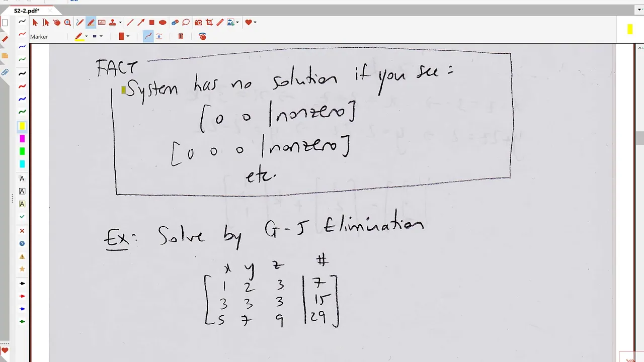



Gaussian Elimination is a systematic method for solving systems of linear equations by transforming an augmented matrix into reduced row echelon form (where the main diagonal contains ones and all other elements are zeros), using three fundamental row operations: row scaling (multiplying a row by a non-zero scalar), row addition (adding one row to another), and row swapping; the process involves creating zeros below the main diagonal through strategic row operations, then scaling rows to make leading coefficients equal to one, ultimately revealing the solution values directly from the right-hand side of the matrix.
Gaussian Elimination: Solve a 2x2 System Step-by-Step | Reduced Row Echelon Form
Added:Understanding of basic algebraic operations and solving simple linear equations with one or two variables.
The geometric interpretation of a 2D linear system, such as lines intersecting, being parallel, or coinciding.
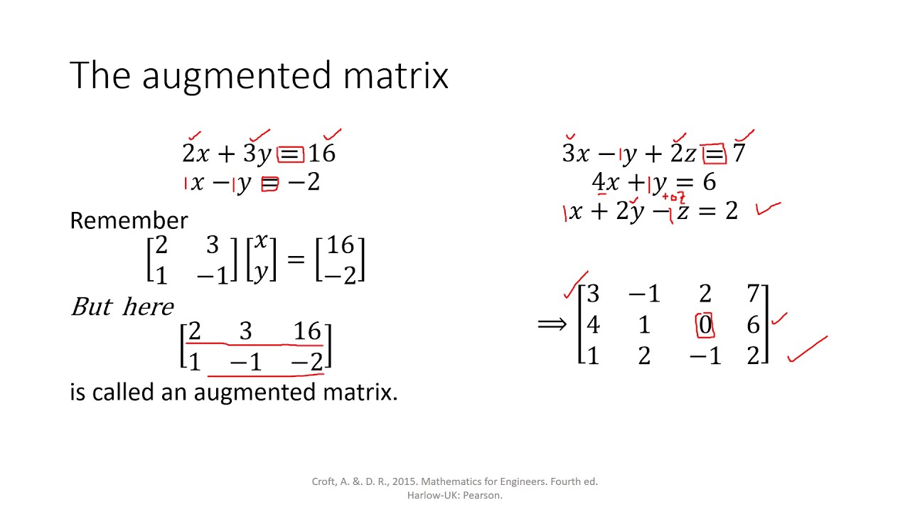
Introduction to matrices, specifically how to represent a system of linear equations as an augmented matrix.
Familiarity with the concept of elementary row operations, such as swapping rows, multiplying a row by a scalar, and adding/subtracting rows.
Applying Gaussian elimination to larger systems of linear equations, such as 3x3 systems and general m x n systems.
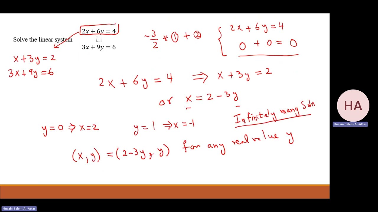
Identifying and interpreting different types of solutions, including unique solutions, infinitely many solutions (introducing free variables), and no solution (inconsistent systems).
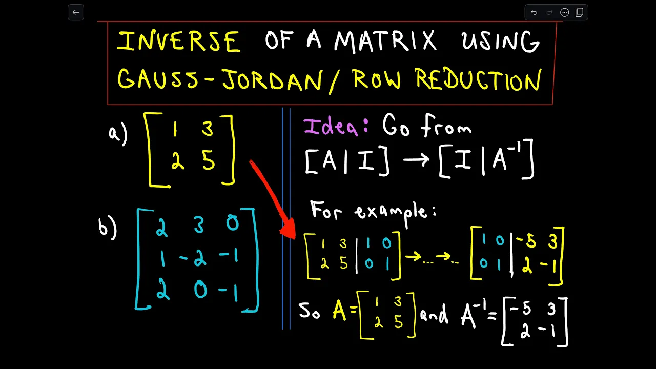
Using Gauss-Jordan elimination to find the inverse of a square matrix.
Exploring real-world applications of linear systems, such as network flow analysis, chemistry equation balancing, and basic computer graphics transformations.
143.1K views1.4Klikes7:18Original Release: 2018-06-24
Hello again everyone. In this video tutorial, we are going to solve this given system of two equations with two variable by Gaussian elimination method.
This method is also called Gaus Jordan elimination method. So let's go ahead and get started with this uh this method. I want you to look at this system of equations. Look at the coefficients over here. Here the coefficient is two. Here no coefficient means by default it's going to be one.
Here is a three and here is a -5. And on the right hand side numbers are -1 and2.
Now I want to transform. I want to put this uh system in a matrix form. So let's go ahead and put in a matrix form.
It's going to look like this thing. We have to be a little bit careful.
Okay. So, I'm going to put a right here the dot dots dots over here. Put down the numbers which is 2 1 3 -5 2 1 35 and -1 and -21 is going to be right up here. By the way, this matrix is called is called augmented matrix. And our now objective is our objective or our goal is to make sure that our this augmented matrix must look like this kind of matrix where we have ones only on the main diagonal. The rest are zeros. If you can see this means that ones are only on the main diagonal. You can see that thing. And on the right hand side we can have x value and y value. So here I have put down my augmented matrix right up here. Now our goal is as I mentioned before we want to make sure that we should have this form. This number should be supposed to be a 1 0 0 1. To achieve that goal, we're going to perform some operations. So these operations I'm going to do. The very first operation is going to be I'm going to multiply the first row, the top row, row number one, multiply by three with row one and put it back on row one. And at the same time, I'm going to multiply the second row by two and put it back to second row. So our this matrix is going to look like so the matrix is going to look like 6 3 -3 and over here it's going to look like -6 10 and 42.
So far so good. And now the next thing what we're going to do is the next operations we're going to do is I want to add first and second row and put it in the second row again. I'm going to put the So this is what I'm going to do. So, I'm going to put down row one and I'm going to add two rows and put it down to a second row R2. So, our matrix is going to look like this one over here. So this is going to become on the top 6 three and again you have to make sure and this is going to be a -3 and here it's going to be a 0 13 and 39.
So far so good. And now as you can see the second row we can easily multiply by 1 over 13. That means we can divide it.
So this is what I'm going to do next one. So I'm going to multiply uh row 1 / 13 times second row and then row two is going to become simply. So once again 6 3 is going to be same and -3 on the top. We not going to touch that one. And the second row is going to simply become 0 1 and this becomes three. So far so good. So the next one we're going to do is we're going to say R1 row 1 - 3 * the second row and put it in a row one the first row. So that's going to look like it's going to look like uh six. I'm going to once again I'm going to put down 6 0 -12 and this is going to stay same 0 1 and 3. And now the final step we are almost finished. I want you to multiply 1 / 6 * row 1 and put it back to row one. So that's going to look like 1 0 -2 and once again make sure so 0 1 and three. So now as you can see this is our x value and this is our y value. And one more thing this 1 0 01 matrix this part only is called reduced row echelon form. In this means that means is that our main diagonal has ones the rest are zero. Thus our solution turns out to be a -2a 3 where -2 is our this x value and 3 is our this y value.
Thanks for watching and please subscribe to my channel for more exciting videos.
Up Next
10:00
행렬식의 기하학적 의미 | 선형대수학의 본질 제6장
@3Blue1BrownKR
40.9K views•2023-10-27

4:43
Elliptic Curve Cryptography Explained: ECC, ECDSA, ECDH
@PracticalNetworking
28.5K views•2024-10-21

10:44
Fourier Series Introduction: The Big Idea Explained
@DrTrefor
387K views•2021-05-03

6:00
The Mathematical Impossibility of Accurate World Maps
@Vox
23.3M views•2016-12-02
Related Study Plans & Knowledge Roadmaps
Structured learning paths in Mathematics
mathematics
Tensor Calculus: Vectors to Riemann Curvature
01Mathematical Foundations: Linear Algebra & Calculus
02Covectors, Dual Spaces, and Tensor Basics
03The Metric Tensor and Index Gymnastics
+ 2 more learning modules
40h5 modules
Explore Roadmap
mathematics
Gödel's Incompleteness: Logic, Proofs & Limits
01Introduction to Formal Systems & Hilbert's Dream
02Set Theory, Cardinality, and Cantor's Diagonal Argument
03Arithmetization and Gödel Numbering
+ 2 more learning modules
14h5 modules
Explore Roadmap
mathematics
Galois Theory: Fields, Groups & Solvability
01Foundations of Abstract Algebra: Groups & Fields
02Polynomials & Field Extensions
03Splitting Fields & Symmetries
+ 2 more learning modules
24h5 modules
Explore Roadmap
mathematics
Non-Euclidean Geometry: Models & Geodesics
01Euclid's Fifth Postulate and the Birth of New Geometries
02Hyperbolic Space and the Poincaré Disk Model
03Geodesics: Defining Straight Lines in Curved Spaces
+ 2 more learning modules
15h5 modules
Explore Roadmap