Consumer surplus is the difference between what consumers are willing to pay and what they actually pay, while producer surplus is the difference between what producers receive and their minimum acceptable price; together, these two surpluses form the total surplus or social welfare, which reaches its maximum at market equilibrium where the sum of both surpluses creates allocative efficiency.
Consumer and Producer Surplus Explained | Microeconomics
Added:Deep Dive
The Law of Demand and how the demand curve represents a consumer's willingness to pay at different price levels.

الفصل الثاني- اقتصاد1 - ECON201 - أ. محمود عامر - نظرية العرض والطلب -الجزء الاول
579
The law of demand states an inverse relationship between price and quantity demanded: as price decreases, quantity demanded increases, and vice versa. A demand curve graphically represents this relationship, always sloping downward from left to right. Price is plotted on the vertical axis and quantity on the horizontal axis. The curve shows how consumers respond to different price levels, demonstrating that higher prices lead to lower quantities demanded and vice versa.
Click to watch →

اقتصاد الباب الثالث - المراجعة النهائية الثانية - الفرقة الاولى
6K
The Law of Demand states there is an inverse relationship between price and quantity demanded: when price decreases, consumers purchase more, and when price increases, they purchase less. This relationship is represented by a downward-sloping demand curve. When price changes, consumers move along the same demand curve (change in quantity demanded). When non-price factors change (income, preferences, prices of related goods), the entire demand curve shifts. Consumer preferences and tastes are key non-price determinants that shift demand.
Click to watch →

مبادئ الإقتصاد الجزئي | المحاضرة 1 | اللقاءات التعليمية | الفصل الأول20231
15K
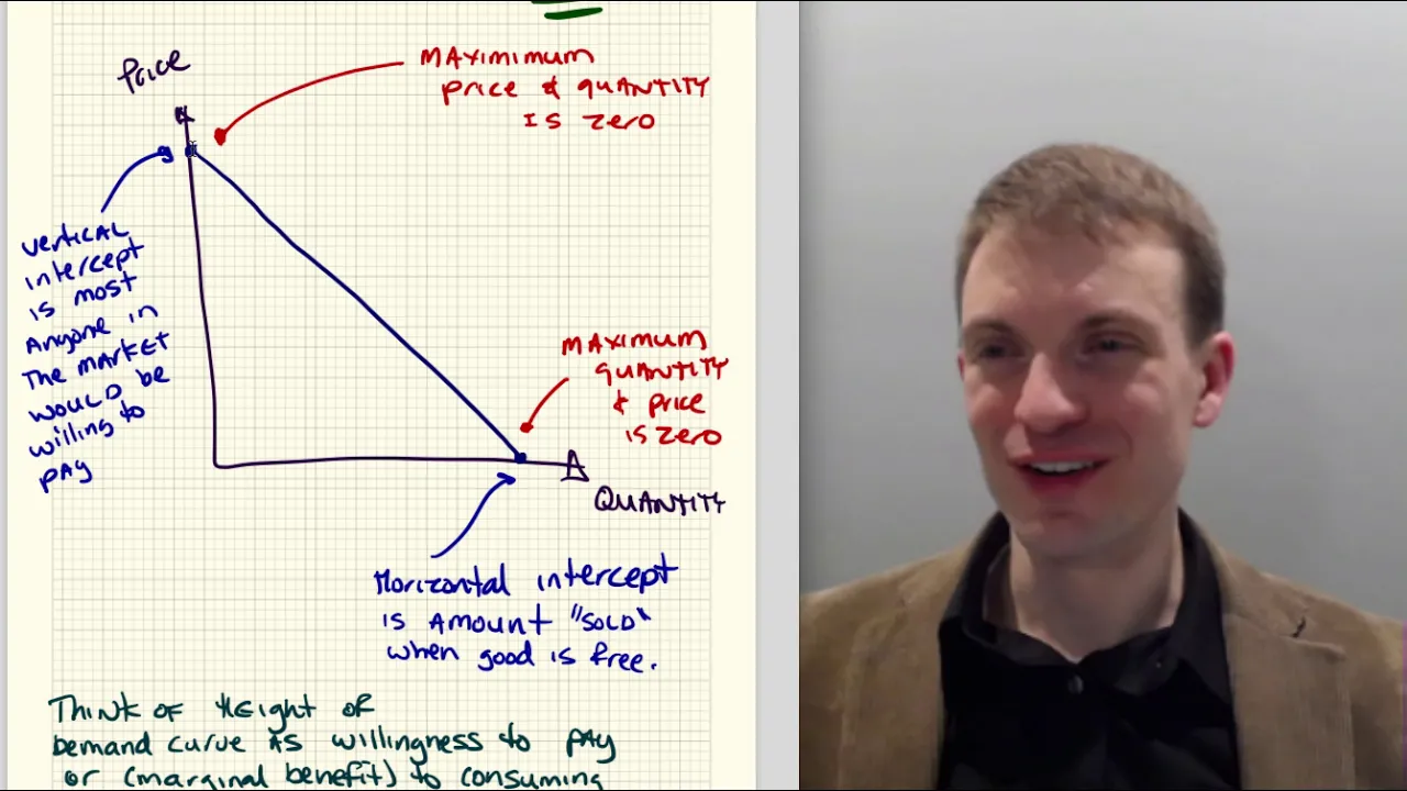
Demand is the quantity consumers are willing and able to purchase at a given price. The Law of Demand states an inverse relationship between price and quantity demanded—when price increases, quantity demanded decreases. This is represented by a downward-sloping demand curve. The curve is typically convex to the origin, meaning the rate of decrease in quantity demanded slows as price increases. This fundamental law helps explain consumer behavior and market equilibrium.
Click to watch →

민성원 국어직강 | 국어 B반 현장 강의 영상 (관세) | 민성원 연구소
5K
This segment explains the law of demand, which states that as the price of a good decreases, the quantity demanded increases, and as the price increases, the quantity demanded decreases. This inverse relationship is represented by a downward-sloping demand curve. The instructor explains that willingness to pay represents the maximum amount a consumer is willing to spend on a good. A consumer will purchase a good if the price is less than or equal to their willingness to pay. Different consumers have different willingness to pay levels based on their preferences, needs, and circumstances. This concept explains why demand curves slope downward - as prices decrease, more consumers find the price acceptable and enter the market.
Click to watch →
![IB Economics Revision Session: Microeconomics [HL/SL]](https://i.ytimg.com/vi/j6Rxiss1qiE/maxresdefault.jpg)
IB Economics Revision Session: Microeconomics [HL/SL]
49.9K
Demand represents the willingness and ability of consumers to purchase a good or service at various prices. The demand curve slopes downward from left to right, illustrating the inverse relationship between price and quantity demanded. This occurs due to three main effects: (1) The wealth effect - when prices fall, consumers feel wealthier and buy more; (2) The marginal utility principle - each additional unit of a good provides less satisfaction than the previous one; (3) The substitution effect - when a good becomes cheaper, consumers substitute it for more expensive alternatives. The law of demand states that as price increases, quantity demanded decreases, and vice versa.
Click to watch →
Deep Dive
The Law of Supply and how the supply curve reflects producers' marginal cost of production.
Supply & Demand Model Explained!
3.2K
The law of supply states that as price rises, quantity supplied rises, and as price falls, quantity supplied falls. The supply curve is typically upward-sloping. The vertical height of the supply curve at any point represents sellers' marginal cost—the minimum price they need to cover production costs. At prices below the supply curve, sellers won't bring goods to market. The vertical intercept shows the minimum price where marginal sellers consider entering the market. Understanding marginal cost explains why suppliers require higher prices to produce additional units.
Click to watch →

Eco 155: Principles of Macroeconomics Class 10
12.2K
Supply is a schedule showing the various amounts of a product that producers are willing and able to bring to market at each specific price during a specified timeframe. The law of supply states that ceteris paribus, as price increases, quantity supplied increases, represented by an upward-sloping supply curve. The height of the supply curve represents marginal cost - how much it costs to produce each additional unit. The first unit costs the least, so it appears at the lowest point. Each successive unit costs more, so the supply curve slopes upward. Production costs vary by location (e.g., wheat costs more to grow in South Florida than Kansas). The supply curve shows the minimum price at which producers are willing to supply each quantity, based on production costs.
Click to watch →

The Supply Curve — From Marginal Cost to Market Supply | Microeconomics
114
This section explains how producers decide how much to produce. A producer's marginal cost (MC) is the cost of producing one more unit. To construct a supply curve, producers track output levels, calculate marginal costs for each new unit, and plot quantity against marginal cost. As production increases, marginal cost typically rises, creating an upward-sloping supply curve. A producer's marginal cost curve is identical to their supply curve because they only sell additional units if the market price covers their production cost. When market prices change, producers move along their existing supply curve. When production costs change (due to labor, materials, or technology), the entire curve shifts. This principle applies universally to all producers, from farmers to tech companies.
Click to watch →
528 Week 1 Part 2b
225
Supply represents producers' willingness and ability to sell goods at various prices, requiring three conditions: resources/technology to produce, profitability potential, and production plans. The law of supply states that higher prices lead to greater quantities supplied, creating an upward-sloping supply curve. This reflects rising marginal costs—the minimum price producers must receive for each additional unit—as production expands. For example, producing the first latte might cost $0.50, but the 50th millionth latte might cost $2.50 due to increased input requirements and resource constraints.
Click to watch →
The Supply Curve is the Marginal Cost Curve
26.2K
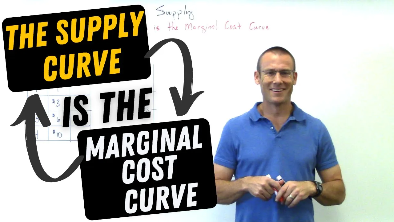
The supply curve is fundamentally the marginal cost curve; firms determine their quantity supplied at each price point by comparing the market price to their marginal cost of production, supplying goods only when price exceeds marginal cost, and shifts in the supply curve occur when input costs change, causing the entire marginal cost curve to shift upward or downward.
Click to watch →
Deep Dive
Market Equilibrium, specifically how the intersection of supply and demand determines market-clearing price and quantity.

Indian Economy for UPSC CSE (IAS): Economic Policy, Supply, Demand, and more - Unacademy
585.4K
Market equilibrium occurs where the market demand curve and market supply curve intersect. At this point, the equilibrium price is the price at which buyers are willing to purchase exactly the quantity that sellers are willing to supply. The equilibrium quantity is the quantity at this intersection. This is also called the market clearing price because at this price, everyone in the market is willing to buy or sell.
Click to watch →

Price determination One shot | Equilibrium Price and Quantity | market equilibrium | Micro economics
58.6K
Market equilibrium occurs when quantity demanded equals quantity supplied, represented by the intersection of demand and supply curves; changes in demand or supply shift the curves and alter equilibrium price and quantity, with demand increases raising both price and quantity, demand decreases lowering both, supply increases lowering price while raising quantity, and supply increases raising price while lowering quantity.
Click to watch →
MBA || SEM 1 || 105 || LECTURE 1 || DEMAND || MANAGERIAL ECONOMICS || THE EDUCATIONAL SHOW
3.8K
Market equilibrium occurs when quantity supplied equals quantity demanded at a specific price. At this point, the demand curve (negative slope) intersects the supply curve (positive slope). Equilibrium price and quantity are determined at this intersection point. This is the market clearing price where consumers can purchase all they want and producers can sell all they want, with no stock piling or shortages.
Click to watch →

equilibrium price and quantity from a given demand and supply function with Graphical depiction
102.9K
Market equilibrium occurs when quantity demanded equals quantity supplied; to find the equilibrium price and quantity mathematically, set the demand function equal to the supply function and solve for price, then substitute the equilibrium price back into either function to find the equilibrium quantity. For example, given QD = 60 - 3P and QS = -40 + 5P, setting 60 - 3P = -40 + 5P yields P = 12.5, and substituting P = 12.5 into either function gives Q = 22.5. Graphically, this is represented by plotting the inverse demand function P = 20 - (Q/3) and inverse supply function P = 8 + (Q/5), where their intersection point shows the equilibrium price and quantity.
Click to watch →

Micro Economics IT Lec16
441
The equilibrium price is the market-clearing price where quantity demanded equals quantity supplied. At this price, the market clears without any tendency to change. The equilibrium quantity is the amount of the good or service that is bought and sold at the equilibrium price. When the market is at equilibrium, both buyers and sellers are satisfied with the transaction price, and there is no pressure for the price to change.
Click to watch →
Prerequisite Knowledge
- Concept 01The Law of Demand and how the demand curve represents a consumer's willingness to pay at different price levels.
- Concept 02The Law of Supply and how the supply curve reflects producers' marginal cost of production.
- Concept 03Market Equilibrium, specifically how the intersection of supply and demand determines market-clearing price and quantity.
Subsequent Learning
- Step 01The concept of Deadweight Loss and how government interventions like price ceilings, price floors, and taxes cause market inefficiencies.
- Step 02How Price Elasticity of Demand and Supply determines the distribution of economic surplus and tax burden (tax incidence).
- Step 03The welfare effects of International Trade, including how tariffs and import quotas alter consumer and producer surplus.
- Step 04Market Failures, such as externalities and monopolies, where unregulated market outcomes fail to maximize total social welfare.
Consumer Surplus
Producer Surplus
Consumer Surplus
0:01Playing Section
- 1
Consumer surplus is the difference between willingness to pay and actual price.
- 2
Surplus varies by individual, with zero surplus for marginal buyers.
- 3
Total surplus is the sum of all individual surpluses.
The Distributional and Equity Critique of Welfare Economics
While standard microeconomics posits that market equilibrium maximizes social welfare by maximizing total (consumer + producer) surplus, critics argue this framework ignores equity and wealth distribution. The traditional surplus model operates on the Kaldor-Hicks efficiency criterion, which treats every dollar of surplus equally, regardless of whether it accrues to a billionaire or a low-income individual. In reality, because of the diminishing marginal utility of wealth, a dollar provides far more utility to a poor person than a rich one. By focusing solely on aggregate efficiency, surplus maximization can justify highly unequal and socially undesirable outcomes. Furthermore, heterodox economists and welfare theorists point out that the model assumes perfect competition and fails to adequately account for externalities, public goods, and market power. Consequently, maximizing total surplus does not guarantee a socially optimal or fair distribution of resources, meaning 'market efficiency' should not be conflated with true societal well-being.
Deep Dive
The concept of Deadweight Loss and how government interventions like price ceilings, price floors, and taxes cause market inefficiencies.

Understanding Deadweight Loss in Economics || Microeconomics || Ugc Net Commerce
3.6K
Deadweight loss is a cost to society created by market inefficiency when supply and demand are not in equilibrium. In imperfect markets, prices become either overvalued or undervalued, leading to inefficient resource allocation. This concept applies to any deficiency caused by inefficient resource allocation. Government interventions such as taxation, price ceilings, and price floors create deadweight loss by preventing markets from reaching equilibrium. When taxes increase, prices rise above equilibrium, reducing demand. Price controls restrict market forces, preventing optimal price discovery. These interventions cause goods to become overvalued or undervalued, changing consumer and producer behavior. The overall economic welfare decreases as resources are misallocated.
Click to watch →

Introductory Microeconomics || Sem - I ||Lecture 002 | Ravindra N Jha || BLISS POINT STUDIES
215
Government interventions such as taxation, price ceilings, and price floors create deadweight loss by reducing total surplus. Deadweight loss represents the loss of economic efficiency that occurs when the equilibrium for a good or service is not achieved. When government interferes with market mechanisms, the total surplus decreases, and this reduction is called deadweight loss. The magnitude of deadweight loss depends on the extent of the intervention.
Click to watch →

Week 5 Part 1
455
Government price controls, including price ceilings (maximum prices) and price floors (minimum prices), create market inefficiencies by reducing the quantity of goods transacted below the equilibrium level, resulting in deadweight loss where mutually beneficial trades no longer occur; while price ceilings benefit some consumers at the expense of suppliers and potentially create black markets, and price floors benefit some producers at the expense of consumers, economists generally argue that direct subsidies or transfers are more efficient ways to support vulnerable groups than intervening in market prices.
Click to watch →

Micro Unit 2 Summary (Old Version)- Supply, Demand, and Consumer Choice
1.1M
Dead weight loss represents inefficiency when markets are not allowed to reach equilibrium. With a price ceiling below equilibrium, consumer surplus increases for some buyers but producer surplus decreases significantly, and dead weight loss appears as an area where potential trades didn't occur. With a price floor above equilibrium, producer surplus increases for some sellers but consumer surplus decreases significantly, with similar dead weight loss. These inefficiencies show that government intervention can reduce total surplus in the economy.
Click to watch →

Microeconomics: Full Course Review for AP & Introductory College
3.7M
Price ceilings and floors create deadweight loss, representing lost economic efficiency. A price ceiling below equilibrium reduces consumer and producer surplus and creates a deadweight loss triangle pointing toward the socially optimal quantity. Similarly, a price floor above equilibrium creates deadweight loss. These interventions prevent the market from reaching its efficient equilibrium.
Click to watch →
Deep Dive
How Price Elasticity of Demand and Supply determines the distribution of economic surplus and tax burden (tax incidence).

New version linked in the description - Microeconomics Unit 2 COMPLETE Summary - Supply and Demand
170K
Tax incidence (who pays the tax) depends on supply and demand elasticities, not who the tax is levied on. The less elastic curve bears more of the tax burden. To determine this: divide the tax revenue box - the top portion represents buyers' loss, the bottom portion represents sellers' loss. Extremes: if supply is perfectly elastic (horizontal), all tax falls on buyers; if demand is perfectly inelastic (vertical), all tax falls on consumers; if supply is perfectly inelastic, all tax falls on sellers.
Click to watch →

NEW- Micro Unit 2 Summary- Supply and Demand
234.9K
Tax incidence refers to who ultimately pays the tax burden. Both buyers and sellers share the tax burden: buyers pay a higher price, and sellers receive a lower price. The distribution depends on elasticity: (1) If demand is more inelastic than supply, consumers pay a larger portion of the tax. (2) If supply is more inelastic than demand, producers pay a larger portion. The more elastic the curve, the less burden it bears.
Click to watch →

Old Version- Micro Unit 2 Summary- Supply and Demand
428.8K
Taxes shift supply curves upward by the tax amount per unit. The tax burden is shared between buyers and sellers based on relative elasticities. If demand and supply have equal elasticity, burden is shared equally. If demand is more inelastic than supply, consumers pay most of the tax. If supply is more inelastic than demand, producers pay most. If demand is perfectly inelastic, consumers pay all the tax. Drawing graphs helps determine who bears the majority of the tax burden.
Click to watch →

Economics(H) Sem I/ Introductory Microeconomics/Demand & Supply 1st Class Incidence
22K
Price Elasticity of Demand is a numerical measure of the degree of responsiveness in quantity demanded due to change in price, keeping other factors constant. There are three types: Price Elasticity of Demand, Income Elasticity of Demand, and Cross Price Elasticity of Demand. The mathematical formula is: Elasticity = (ΔQ/ΔP) × (P/Q). Price and quantity demanded have an inverse relationship, so elasticity is always negative. On a straight line demand curve, elasticity varies between zero and infinity - at the vertical end (price = 0), elasticity is zero (perfectly inelastic); at the horizontal end (quantity = 0), elasticity is infinity (perfectly elastic). Tax incidence refers to the burden of tax on buyers and sellers. The burden depends on elasticity: Buyer's Burden ∝ Elasticity of Supply / Elasticity of Demand, and Seller's Burden ∝ Elasticity of Demand / Elasticity of Supply. When tax is imposed, the supply curve shifts upward (if on sellers) or demand curve shifts downward (if on buyers), creating a wedge between the price buyers pay and the price sellers receive. The gap equals the tax size. Government tax revenue equals tax per unit multiplied by quantity sold after tax.
Click to watch →

KINH TẾ VI MÔ - TỔNG ÔN CUỐI KỲ - CHỮA TRẮC NGHIỆM CUNG CẦU CHI TIẾT
21.7K
This section covers tax incidence and elasticity. Key topics include: (1) Tax incidence (who bears the burden of tax) depends on relative elasticities of supply and demand; (2) The more inelastic side bears more of the tax burden; (3) When demand is perfectly inelastic (vertical demand curve), consumers bear the entire tax burden; (4) When supply is perfectly inelastic, producers bear the entire tax burden; (5) Price elasticity of demand (PED) measures responsiveness: PED = (%ΔQ) / (%ΔP); (6) For example, if price decreases by 20% and quantity demanded increases by 40%, PED = 40/(-20) = -2; (7) When demand is perfectly elastic (horizontal demand curve), producers bear the entire tax burden; (8) Tax burden distribution depends on relative elasticities - the more inelastic side bears more of the tax burden; (9) When taxes are imposed on sellers, the supply curve shifts left, equilibrium price increases and equilibrium quantity decreases; (10) The magnitude of equilibrium changes depends on the relative elasticities of supply and demand.
Click to watch →
Deep Dive
The welfare effects of International Trade, including how tariffs and import quotas alter consumer and producer surplus.

Микроэкономика 9. Долгосрочный анализ конкурентного рынка. Налоговое бремя. Международная торговля
117
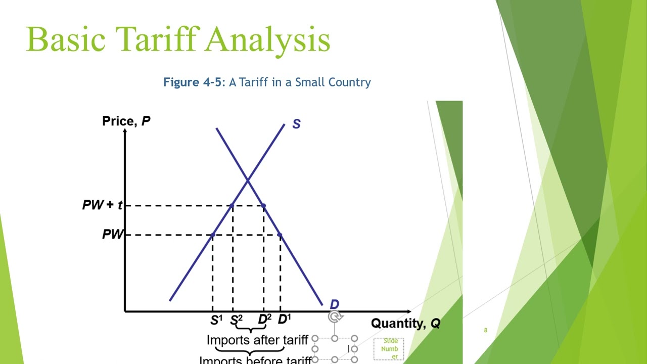
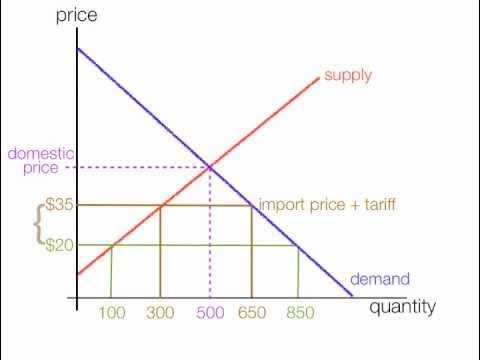
A tariff is a tax on imported goods that raises the domestic price of imported goods. When a tariff is imposed, the domestic price rises, reducing consumer surplus and increasing producer surplus. The government collects tariff revenue equal to the tariff rate times the quantity of imports. The net welfare effect is negative due to deadweight loss triangles on both sides of the market. An import quota is a quantitative restriction on the amount of goods that can be imported. A quota has similar effects to a tariff on domestic prices and quantities, but the welfare distribution differs. The quota rent goes to whoever holds the import licenses, which may be foreign producers or domestic importers.
Click to watch →

2004 AP Micro FRQ#2 (World Price/Tariff)
1.1K
International trade creates winners and losers in the economy through changes in consumer and producer surplus. Consumer surplus increases substantially when prices fall to the world level, expanding from the area above P2 to the area above Pw, capturing additional benefits for consumers. Conversely, producer surplus decreases as producers receive lower prices and produce less output. The net effect on national welfare depends on comparing these changes. The net gain from trade represents the total welfare improvement, calculated as the difference between post-trade and pre-trade total surplus, typically appearing as an additional triangular area in the demand-supply diagram.
Click to watch →

Tariffs and Quotas
1.4K
Like tariffs, quotas result in a loss of consumer surplus (areas 1, 2, 3, and 4) because the domestic price increases. Area 1 represents the gain in domestic producer surplus, as domestic producers benefit from the higher price and increased sales. Area 3 is different from tariffs because it represents the extra revenue that lucky importers receive (P- minus PW) for the right to import under the quota. This quota rent goes to importers who have obtained the import licenses, rather than to the government as with tariffs.
Click to watch →
section 20 international trade
342
Consumer surplus represents the difference between what consumers are willing to pay and what they actually pay, shown graphically as the area between the demand curve and price line. Producer surplus is the difference between the price received and the minimum acceptable price, shown as the area between the supply curve and price line. Tariffs reduce consumer surplus while increasing producer surplus in importing countries, redistributing welfare from consumers to domestic producers and government.
Click to watch →

M-14. Tariffs, partial equilibrium analysis of tariff, effect on producer and consumer surplus
566
Consumer surplus represents the difference between what consumers are willing to pay and what they actually pay, measured as the area below the demand curve and above the market price. Producer surplus represents the difference between what producers receive and their minimum acceptable price, measured as the area above the supply curve and below the market price. When tariffs raise prices, consumer surplus decreases because consumers pay more for the same quantity. Conversely, producer surplus increases as domestic producers sell at higher prices. These concepts provide essential tools for measuring welfare effects in international trade, allowing economists to quantify how trade policies redistribute economic benefits between consumers and producers.
Click to watch →
Deep Dive
Market Failures, such as externalities and monopolies, where unregulated market outcomes fail to maximize total social welfare.

6.3 Market Failures and Externalities
7.5K
The competitive market equilibrium is assumed to be welfare maximizing, but this assumption leads to an uncomfortable conclusion: that aside from redistribution, there should be no government involvement. However, government intervention is widespread (military spending, environmental regulation). Market failures explain why free markets don't always achieve efficient outcomes. One major source is market power in monopolies/oligopolies. Another is externalities—situations where actions affect others without compensation. Negative externalities (like pollution) cause overproduction because actors ignore harm to others. Positive externalities cause underproduction because actors ignore benefits to others. The goal is to maximize social welfare by ensuring decisions account for all affected parties.
Click to watch →

LDV - Introducción a la Economía (EAE105A) / Derecho
1.1K
Externalities represent market failures because the market equilibrium does not maximize total social welfare. In the case of negative externalities, the market produces too much of the good because producers do not bear all the costs of their actions. In the case of positive externalities, the market produces too little because producers do not receive all the benefits of their actions. Government intervention (like taxes for negative externalities or subsidies for positive externalities) can help correct these market failures.
Click to watch →

Externalities and market failure
2.1K
Market failure occurs when an unregulated market fails to produce an outcome that is most beneficial to society as a whole. Externalities are a primary cause of market failure because private market transactions do not account for all social costs and benefits, leading to inefficient resource allocation.
Click to watch →

Falhas de Mercado I
286
Market failures prevent the First Welfare Theorem from achieving Pareto efficient equilibrium. Well-defined property rights require universality, complete specification, no information asymmetry, and contractual exclusivity, with rights transferable and protected from confiscation. Market power occurs when participants influence prices, arising from barriers to entry like legal restrictions, patents, or resource control. Natural monopolies emerge from high fixed costs and economies of scale. The monopolist maximizes profit where Marginal Revenue equals Marginal Cost, producing less and charging more than perfect competition. The price formula P = MC / (1 + 1/|E|) shows monopolists only produce where demand is elastic. Externalities occur when production or consumption affects third parties not involved in the transaction, with effects not transmitted through market prices. In negative externalities, private supply lies below social supply, causing overproduction. In positive externalities, private demand lies below social demand, causing underproduction. The socially optimal quantity occurs where Marginal Social Cost equals Marginal Social Benefit.
Click to watch →

Externalities | Chapter 10 | Mankiw Principles of Microeconomics 8th ed.
2K
Markets are good at organizing economic activity because they maximize total surplus (consumer surplus + producer surplus). However, when externalities exist, the market equilibrium cannot maximize total benefit to society. This represents a type of market failure where the market outcome is not efficient.
Click to watch →
Consumer Surplus
Producer Surplus
Consumer Surplus
0:01- 1
Consumer surplus is the difference between willingness to pay and actual price.
- 2
Surplus varies by individual, with zero surplus for marginal buyers.
- 3
Total surplus is the sum of all individual surpluses.
The Distributional and Equity Critique of Welfare Economics
While standard microeconomics posits that market equilibrium maximizes social welfare by maximizing total (consumer + producer) surplus, critics argue this framework ignores equity and wealth distribution. The traditional surplus model operates on the Kaldor-Hicks efficiency criterion, which treats every dollar of surplus equally, regardless of whether it accrues to a billionaire or a low-income individual. In reality, because of the diminishing marginal utility of wealth, a dollar provides far more utility to a poor person than a rich one. By focusing solely on aggregate efficiency, surplus maximization can justify highly unequal and socially undesirable outcomes. Furthermore, heterodox economists and welfare theorists point out that the model assumes perfect competition and fails to adequately account for externalities, public goods, and market power. Consequently, maximizing total surplus does not guarantee a socially optimal or fair distribution of resources, meaning 'market efficiency' should not be conflated with true societal well-being.
The Law of Demand and how the demand curve represents a consumer's willingness to pay at different price levels.
The Law of Supply and how the supply curve reflects producers' marginal cost of production.
Market Equilibrium, specifically how the intersection of supply and demand determines market-clearing price and quantity.
The concept of Deadweight Loss and how government interventions like price ceilings, price floors, and taxes cause market inefficiencies.
How Price Elasticity of Demand and Supply determines the distribution of economic surplus and tax burden (tax incidence).
The welfare effects of International Trade, including how tariffs and import quotas alter consumer and producer surplus.
Market Failures, such as externalities and monopolies, where unregulated market outcomes fail to maximize total social welfare.
97.9K views1.7Klikes3:22@economicsmafiaOriginal Release: 2015-02-05
What exactly is consumer surplus?
Suppose I want a computer because it gives me a happiness of $700 I go to the market and realize I can buy it at just $500 Woohoo! $200 of net happiness This is my consumer surplus On the demand curve Though everyone pays the same price at $500 different consumers have different willingness to pay I'm willing to get the computer at $700 It costs only $500 My surplus is $200 Then another guy is willing to pay $600 His surplus is lower, at $100 And of course you have a guy who's only willing to pay $500 His surplus is $0 What about a guy who's willing to pay $400?
The computer costs $500!
No transaction will take place Add up all these surpluses, this is the total consumer surplus in the market What about producer surplus?
Suppose I produce computers I want to sell each of these at $300 I go to the market and realize that everyone else is selling these at $500 Happily, I price my computer at $500 Which is cool!
I'm expecting $300 but I get $500 That's $200 extra On the supply curve Though everyone sells at the equilibrium price of $500 different producers have different willingness to sell I hope to sell my computer for at least $300 Sold it at $500 My producer surplus is $200 Another guy wants to sell his computer at $400 His surplus will be lower at $100 For a guy who's wants to sell his computer at $500 His producer surplus is $0 Add up all the producer surplus And you get a triangle area Add up these 2 triangles We have the total surplus Also known as the social welfare All of us know that this is the market equilibrium point Do you know this is also the allocatively efficient point?
Check out the next video on Allocative Efficiency If you like this video, remember to like and subscribe
Up Next
6:44
Tariff Impact on Consumer Surplus, Producer Surplus, & Deadweight Loss
@economicsfun
333.7K views•2010-11-13

5:07
Impact of Yuan in Indo-Russian Trade Amid Sanctions
@WION
261.9K views•2022-07-01
10:33
Behavioral Economics Explained: Rationality, Nudges, and Risk
@crashcourse
1.1M views•2016-03-12

113:18
The Age of Easy Money: Fed & Inflation | Full Documentary
@frontline
21.2M views•2023-03-15
Related Study Plans & Knowledge Roadmaps
Structured learning paths in Economics
economics
Sovereign Debt: Defaults, IMF & Restructuring
01Introduction to Sovereign Debt & Government Bonds
02Debt Sustainability & Credit Ratings
03Anatomy and History of Debt Crises
+ 2 more learning modules
12h5 modules
Explore Roadmap
economics
Market Design: Matching Theory & Gale-Shapley
01Introduction to Market Design and Price-Free Markets
02Two-Sided Matching & The Gale-Shapley Algorithm
03School Choice Systems and Mechanism Design
+ 2 more learning modules
10h5 modules
Explore Roadmap
economics
Impossible Trinity: Forex, Capital & Policy
01Introduction to Monetary Policy and Central Banking
02Exchange Rates and International Capital Flows
03The Mundell-Fleming Model
+ 2 more learning modules
8h5 modules
Explore Roadmap
economics
Healthcare Economics: Market Failures & Systems
01Introduction to Healthcare Markets and Market Failure
02Asymmetric Information and Adverse Selection
03Moral Hazard and Insurance Design
+ 2 more learning modules
12h5 modules
Explore Roadmap