To find the minimal polynomial of an algebraic element over the rationals, first express the element as α, perform algebraic manipulations to derive a polynomial equation with rational coefficients that α satisfies, then verify irreducibility using criteria like Eisenstein's criterion; if the polynomial is monic and irreducible, it is the minimal polynomial. For example, for α = 2 - ∛5, we find that α satisfies (x - 2)³ + 5 = 0, which is irreducible by Eisenstein's criterion applied to x³ + 5 with p = 5, and since shifting a polynomial preserves irreducibility, this confirms it is the minimal polynomial.
Minimal Polynomial of 2 - Cube Root of 5 over Q
Added:Deep Dive
Definition of algebraic elements, algebraic numbers, and the formal definition of a minimal polynomial over the field of rational numbers (Q).

高校数学からガロア理論へ:代数的数による有理数の拡大
211
An algebraic number is a complex number that is a root of some polynomial with rational coefficients. Examples include √2 (root of x²-2) and i (root of x²+1). A transcendental number cannot be a root of any rational polynomial, like π and e. The minimal polynomial of an algebraic number α is the unique polynomial with rational coefficients that has α as a root, has the smallest possible degree, and has leading coefficient 1. This polynomial is always unique and irreducible over the rationals.
Click to watch →

Field Theory || Abstract Algebra || Minimal Polynomial of elements over Field ||By Mr. Parveen Kumar
5.7K
The minimal polynomial of an algebraic element α over a field F is the monic polynomial of least degree in F[x] that is irreducible over F and has α as a root; for example, the minimal polynomial of √3 over Q is x² - 3, and for a primitive nth root of unity over Q, it is the cyclotomic polynomial Φₙ(x) of degree φ(n).
Click to watch →

FIELD THEORY 1 | INTRODUCTORY LECTURE | MANISH SIR | #fieldtheory #csirnetmaths #gate
3K
An element α is algebraic over F if some non-zero polynomial in F[x] has α as a root. An extension is algebraic if all its elements are algebraic over F. The minimal polynomial of α over F is the unique monic irreducible polynomial m(x) such that m(α) = 0. It is the polynomial of lowest degree with α as a root. The degree of m(x) equals [F(α):F]. Any polynomial with α as a root is divisible by m(x). Examples: minimal polynomial of √2 over Q is x² - 2; of ∛2 over Q is x³ - 2.
Click to watch →
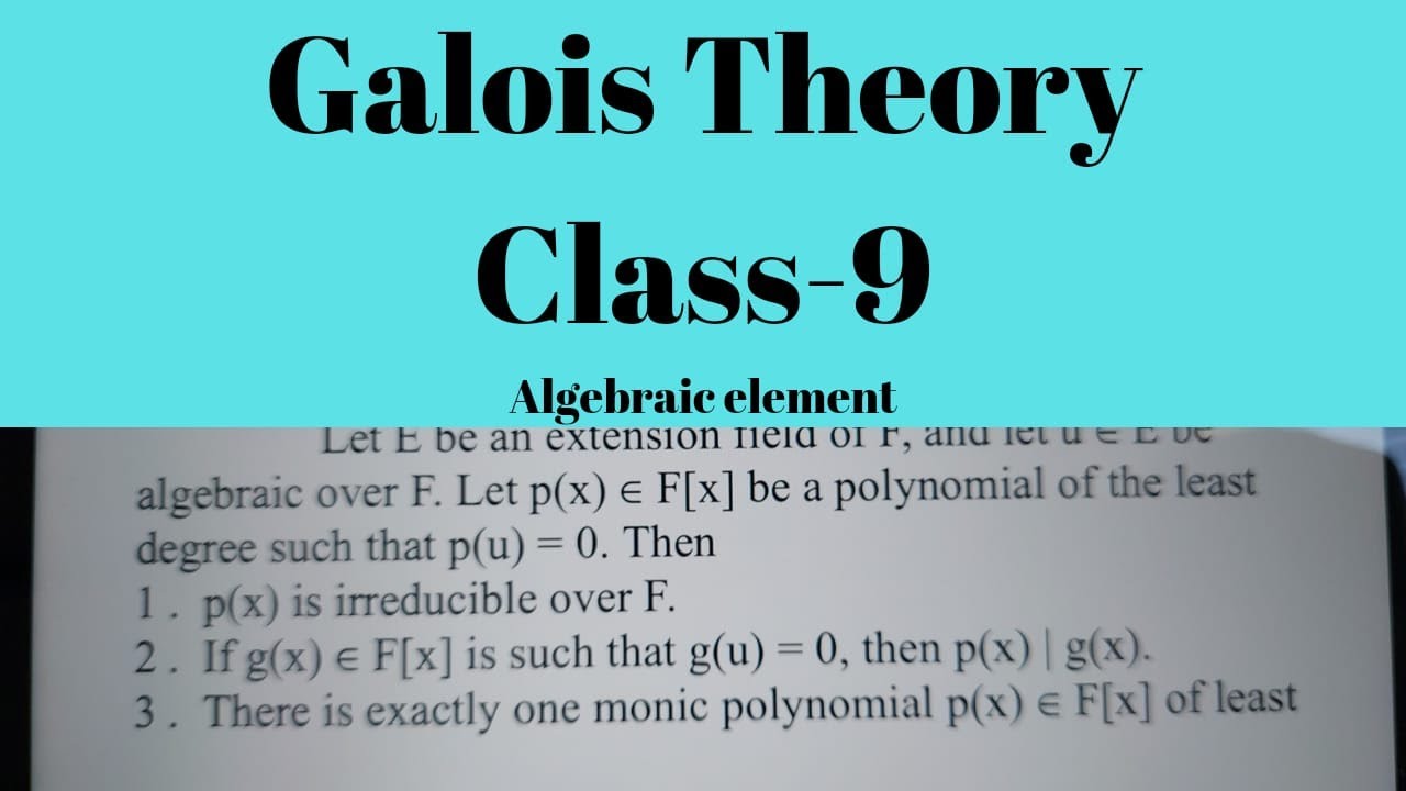
Galois Theory - Class - 9 : Algebraic element
737
An element α in an extension field E of a field F is algebraic over F if there exists a non-zero polynomial f(x) with coefficients in F such that f(α) = 0. The minimal polynomial of α is defined as the monic polynomial of least degree in F[x] that has α as a root. This concept forms the foundation for understanding algebraic extensions and their properties.
Click to watch →

Why are Most Polygons Impossible to Construct?
55K
The minimal polynomial of an algebraic number α is the monic polynomial of least degree with rational coefficients for which α is a root. It is unique and irreducible. If α satisfies a polynomial equation with rational coefficients, then its minimal polynomial divides that polynomial. The degree of the minimal polynomial equals the degree of the field extension Q(α) over Q.
Click to watch →
Deep Dive
Understanding polynomial irreducibility and how to apply Eisenstein's Criterion to prove irreducibility over Q.
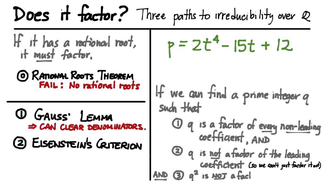
302.S1: Three Paths to Irreducibility
23.4K
Eisenstein's criterion provides a powerful method to prove a polynomial is irreducible over Q. The criterion requires finding a prime number p such that: (1) p divides every non-leading coefficient of the polynomial, (2) p does not divide the leading coefficient, and (3) p² does not divide the constant term. When these three conditions are satisfied, the polynomial is guaranteed to be irreducible over Q. The key insight is that if such a prime exists, any attempted factorization would require both factors to have coefficients divisible by p, leading to a contradiction since the constant term would then be divisible by p².
Click to watch →
How to make new fields -- Abstract Algebra 24
4.8K
Eisenstein's Criterion provides a test for irreducibility over Q: Let p be a prime, and let f(x) = aₙxⁿ + ... + a₁x + a₀. If p divides all coefficients a₀ through aₙ₋₁, p does not divide aₙ, and p² does not divide a₀, then f(x) is irreducible over Q. Proof by contradiction: Assume f(x) = A(x)B(x) with A,B ∈ Q[x]. By Gauss's Lemma, A,B ∈ Z[x]. Let m be minimal index where p ∤ bₘ (coefficient of A). Then coefficient aₘ = Σₖ bₖcₘ₋ₖ, where b₀,...,bₘ₋₁ divisible by p, but bₘ not divisible by p, and c₀ not divisible by p (since p ∤ a₀). Thus aₘ is not divisible by p, contradicting that p divides all aᵢ for i < n.
Click to watch →

Irreducible Polynomials
29.5K
Eisenstein's Criterion provides a sufficient condition for a polynomial to be irreducible over ℚ[X]. For a polynomial f = cₙxⁿ + ... + c₁x + c₀ with integer coefficients, if there exists a prime p such that: (1) p does not divide cₙ, (2) p divides all other coefficients cₙ₋₁, ..., c₁, c₀, and (3) p² does not divide c₀, then f is irreducible over ℚ[X]. The proof proceeds by contradiction, assuming a factorization exists and showing that p must divide all coefficients including the leading one, which contradicts condition (1).
Click to watch →

CSIR NET & SET: Examples for Irreducible Polynomials Ring Theory Maths
8.4K
Eisenstein's Criterion provides a powerful method to prove irreducibility: For f(x) = a₀ + a₁x + ... + aₙxⁿ in Z[x], if there exists a prime p such that p divides all coefficients except the leading one, p does not divide the leading coefficient, and p² does not divide the constant term, then f(x) is irreducible over Q. This criterion is essential for proving irreducibility of many polynomials.
Click to watch →

Critério de Eisenstein (polinômios) - Prof. Adriano Carneiro
7.6K
Eisenstein's Criterion states that for a polynomial P(x) = a_n x^n + a_{n-1} x^{n-1} + ... + a_1 x + a_0 with integer coefficients, if there exists a prime number p such that p divides all coefficients a_0 through a_{n-1}, p does not divide the leading coefficient a_n, and p^2 does not divide the constant term a_0, then the polynomial is irreducible over the rational numbers. This criterion provides a powerful method to prove polynomial irreducibility without attempting factorization.
Click to watch →
Deep Dive
Basic algebraic manipulation techniques to isolate and eliminate radical terms (such as cube roots) from equations.

السادس العلمي/الفصل الثالث/محاضرة 33/التقريب الجزء السادس
156K
The instructor demonstrates algebraic manipulation to isolate the variable r. The equation 84 = (4/3)r³ is rearranged by multiplying both sides by 3 and dividing by 4, resulting in r³ = 63. The instructor explains that this step eliminates the coefficient (4/3) from the r³ term, leaving r³ = 63. This is a crucial step before applying the cube root.
Click to watch →
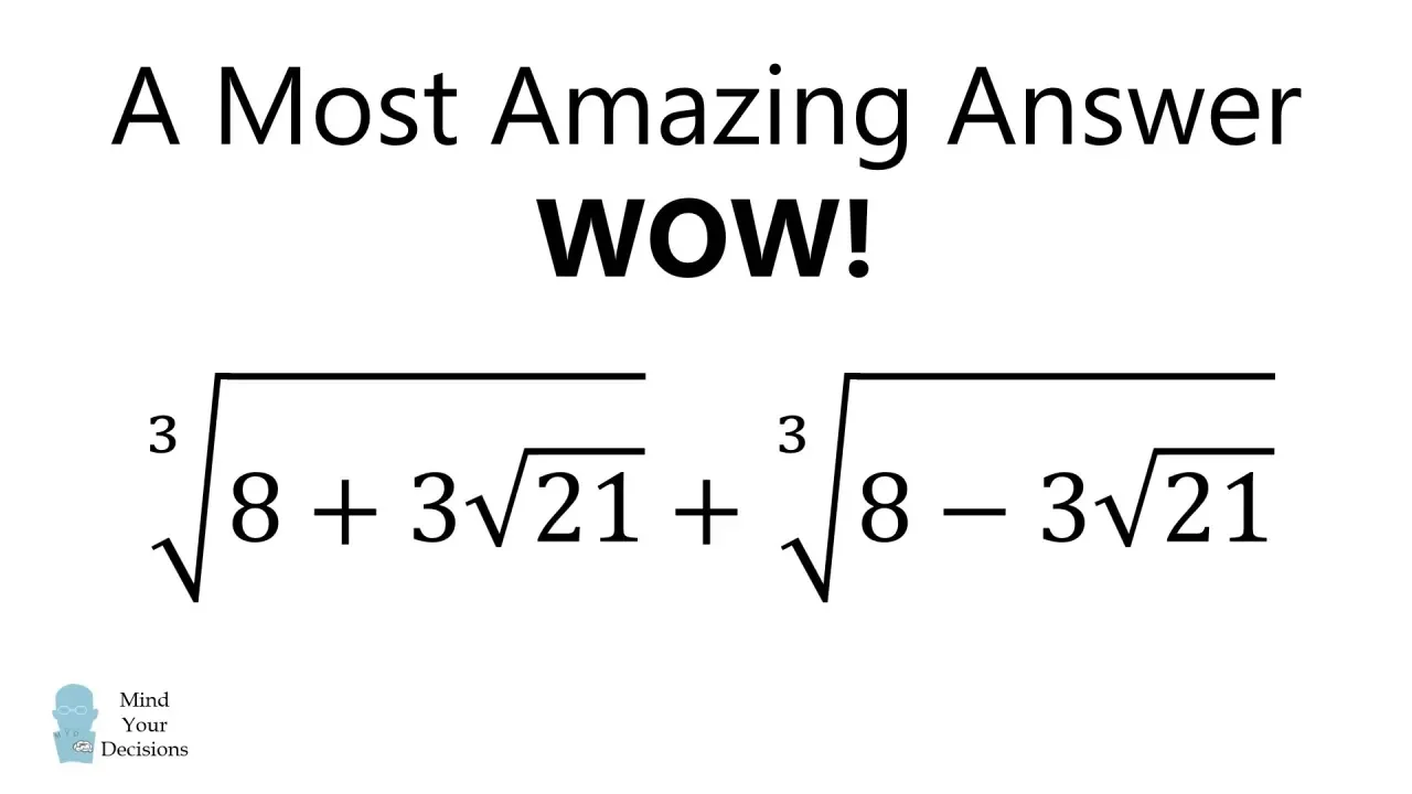
WOW! A Most Amazing Answer
860.1K
To simplify an expression containing cube roots, set the entire expression equal to a variable (x), then cube both sides of the equation. This algebraic manipulation eliminates the cube roots and transforms the problem into a polynomial equation that can be solved using standard algebraic techniques.
Click to watch →

A Nice Math Olympiad Problem | You should know this trick!
123
This segment demonstrates the systematic process of isolating and eliminating radicals from algebraic equations. The instructor shows how to move constant terms to isolate the radical expression, then divide by coefficients to simplify. The key step involves cubing both sides to eliminate the cube root, converting the equation from radical form to polynomial form. This transformation allows the equation to be solved using standard algebraic techniques for polynomial equations.
Click to watch →

Algebra Rare Identities Explained 🔥| Every Student Must Know (with Top SSC Ques.) | Bhutesh Sir
624
When equations contain cube roots, cubing both sides eliminates the radicals and simplifies the expression. Starting with x^(1/3) + y^(1/3) + z^(1/3) = 0, cubing yields x + y + z + 3(x^(1/3) + y^(1/3) + z^(1/3))(x^(1/3)y^(1/3) + y^(1/3)z^(1/3) + z^(1/3)x^(1/3)) = 0. Since the sum of cube roots equals zero, the entire second term vanishes, leaving x + y + z = 0. This technique transforms complex radical expressions into polynomial equations that are easier to solve and analyze.
Click to watch →

Raiz cúbica de radical duplo
35K
To simplify a cube root expression, one can apply algebraic manipulations by cubing both sides of the equation. When the cube root is cubed, the index (3) cancels out with the exponent (3), effectively removing the radical. This technique allows the expression to be transformed into a polynomial form that can be compared with the desired simplified form.
Click to watch →
Deep Dive
The concept of polynomial rings, specifically Q[x], and the division algorithm for polynomials.

Lec 18 | Polynomial Ring | Division algorithm of Polynomials
426
The division algorithm for polynomials states that for any polynomial f(x) and any non-zero polynomial g(x), there exist unique polynomials q(x) (quotient) and r(x) (remainder) such that f(x) = g(x)q(x) + r(x), where the degree of r(x) is less than the degree of g(x). This algorithm is fundamental in polynomial rings and allows for the systematic division of polynomials, similar to integer division.
Click to watch →

DSSSB TGT/PGT MATHS | Ring Theory | Polynomial Ring Part-2 | By Romika Bhargav
2.1K
The Division Algorithm for polynomials states that for any polynomial f(x) and non-zero polynomial g(x) over a field F, there exist unique polynomials q(x) (quotient) and r(x) (remainder) such that f(x) = g(x)q(x) + r(x), where either r(x) = 0 or the degree of r(x) is less than the degree of g(x). This is analogous to integer division where dividend = divisor × quotient + remainder.
Click to watch →
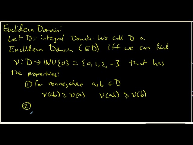
87 Definition of Euclidean Domain
174
For a field F, the ring of polynomials F[x] has a division algorithm: if f and g are in F[x] and g ≠ 0, then there exist polynomials q and r in F[x] such that f = qg + r, where either the degree of r is strictly less than the degree of g, or r is identically zero.
Click to watch →
Polynômes et évaluations à l'agrégation interne
2K
The division algorithm guarantees that for any P(X) and non-zero A(X), there exist unique Q(X) and R(X) with P(X) = A(X)Q(X) + R(X) and deg(R) < deg(A). This enables construction of quotient rings K[X]/(A). The remainders serve as canonical representatives of equivalence classes. The set {1, X, X², ..., X^{d-1}} forms a basis for the quotient ring where d = deg(A), providing a concrete realization of abstract quotient structures.
Click to watch →
![L 29 Example of Quotient Ring | Z[i]/(2-i) | Ring theory and Linear Algebra 1 | B Sc Hons Maths | DU](https://i.ytimg.com/vi/Aewq-0v372Q/maxresdefault.jpg)
L 29 Example of Quotient Ring | Z[i]/(2-i) | Ring theory and Linear Algebra 1 | B Sc Hons Maths | DU
4.5K
This segment covers polynomial rings and the division algorithm for polynomials. The instructor explains how polynomial rings can be quotiented by ideals to create new algebraic structures, and demonstrates how the division algorithm applies to polynomial rings. The video shows how to divide one polynomial by another to express it as a quotient plus a remainder, where the remainder has lower degree than the divisor. The instructor emphasizes that this algorithm is fundamental for working with polynomial rings and is used to simplify expressions and determine equivalence classes in polynomial quotient rings.
Click to watch →
Prerequisite Knowledge
- Concept 01Definition of algebraic elements, algebraic numbers, and the formal definition of a minimal polynomial over the field of rational numbers (Q).
- Concept 02Understanding polynomial irreducibility and how to apply Eisenstein's Criterion to prove irreducibility over Q.
- Concept 03Basic algebraic manipulation techniques to isolate and eliminate radical terms (such as cube roots) from equations.
- Concept 04The concept of polynomial rings, specifically Q[x], and the division algorithm for polynomials.
Subsequent Learning
- Step 01Determining the degree of simple algebraic field extensions [Q(alpha) : Q] using the degree of the minimal polynomial of alpha.
- Step 02Constructing explicit vector space bases for simple algebraic field extensions (e.g., finding a basis for Q(2 - 5^(1/3)) over Q).
- Step 03Finding minimal polynomials for more complex algebraic numbers involving multiple distinct radicals, such as the sum of square roots and cube roots.
- Step 04Exploring Galois Theory, including identifying the splitting field of the minimal polynomial and calculating its Galois group.
Finding Minimal Polynomial
Finding Minimal Polynomial
0:00Playing Section
- 1
Define alpha as the root of the shifted cubic polynomial.
- 2
Derive polynomial by cubing the shifted expression for alpha.
- 3
Confirm polynomial is monic and irreducible for minimality.
The Resultant and Galois-Theoretic Approach
While using a cubic shift and Eisenstein's criterion offers an intuitive, hands-on method for finding the minimal polynomial of 2 - 5^(1/3), this ad-hoc approach lacks scalability for more complex algebraic numbers. A powerful alternative perspective is the systematic use of Field Theory and Resultants. By viewing the problem through field extensions and the tower law, or by computing the polynomial resultant of x - (2 - y) and y^3 - 5, mathematicians can algorithmically determine minimal polynomials. This systematic approach avoids the need for clever algebraic manipulations and generalizes to any combination of algebraic elements, shifting the focus from elementary arithmetic tricks to structural, algorithmic algebra.
Deep Dive
Determining the degree of simple algebraic field extensions [Q(alpha) : Q] using the degree of the minimal polynomial of alpha.
Abstract Algebra II: algebraic extensions, 1-24-18
586
For an algebraic element α over F, the degree of the simple extension F(α) over F equals the degree of the minimal polynomial of α over F. This is a direct consequence of the fact that F(α) is isomorphic to F[X]/(m_α,F(X)), and the degree of this quotient ring as a vector space over F is exactly the degree of the polynomial m_α,F(X). This provides a concrete way to compute the degree of field extensions generated by algebraic elements.
Click to watch →

7: Algebraische Körpererweiterungen
413
If f(x) is the minimal polynomial of α over K with degree d, then [K(α):K] = d. This means the degree of the simple algebraic extension equals the degree of the minimal polynomial of the adjoined element.
Click to watch →

【ガロア理論】代数閉体と代数閉包
3.2K
Let E/F be a field extension and α ∈ E be algebraic over F. The simple extension F(α) is isomorphic to F[x]/(P(x)), where P(x) is the minimal polynomial of α over F. The degree [F(α):F] equals the degree of P(x). This shows that algebraic simple extensions are finite and determined by the minimal polynomial of the adjoined element.
Click to watch →
Lecture 9 The degree of a field extension (part 1)
306
If α is algebraic over F with minimal polynomial of degree D, then the set {1, α, α², ..., α^(D-1)} forms a basis for F(α) as a vector space over F. This provides an explicit basis for all simple algebraic extensions. For Q(∛2), the basis is {1, ∛2, (∛2)²}. For Q(√5), the basis is {1, √5}. For Q(ζ₃), the basis is {1, ζ₃}. The number of basis elements equals the degree of the minimal polynomial.
Click to watch →

Estudio de un elemento algebraico o trascendente sobre los racionales | Álgebra | UNED
381
The degree of the field extension Q(α) over Q equals the degree of the minimal polynomial of α. Since the minimal polynomial has degree 4, [Q(α):Q] = 4. This means α generates a field extension of dimension 4 over the rationals, which is a fundamental result in field theory.
Click to watch →
Deep Dive
Constructing explicit vector space bases for simple algebraic field extensions (e.g., finding a basis for Q(2 - 5^(1/3)) over Q).
Lecture 9 The degree of a field extension (part 1)
306
If α is algebraic over F with minimal polynomial of degree D, then the set {1, α, α², ..., α^(D-1)} forms a basis for F(α) as a vector space over F. This provides an explicit basis for all simple algebraic extensions. For Q(∛2), the basis is {1, ∛2, (∛2)²}. For Q(√5), the basis is {1, √5}. For Q(ζ₃), the basis is {1, ζ₃}. The number of basis elements equals the degree of the minimal polynomial.
Click to watch →

Lección 16 - Extensiones de cuerpos simples | Álgebra | UNED
519
For a simple algebraic extension L = K(α) over K, the degree [L:K] equals the degree of the minimal polynomial of α over K. If the minimal polynomial has degree n, then a basis for L as a K-vector space is {1, α, α², ..., α^(n-1)}. This provides complete information about the extension's structure. For Q(√2) over Q, the minimal polynomial is t² - 2, degree 2, and basis is {1, √2}. Complex extensions can be studied as towers of simple extensions: for K ⊆ M ⊆ L, if L/M and M/K are finite, then [L:K] = [L:M] × [M:K]. For Q(√2, √3) over Q, we have Q(√2) over Q (degree 2) and Q(√2, √3) over Q(√2) (degree 2), giving total degree 4 with basis {1, √2, √3, √6}.
Click to watch →

2. О симметрических многочленах и алгебраических числах
209
For α = 2 + ∛5 with degree 3, the field extension Q(α) has dimension 3 over Q. A basis is constructed by taking powers of α from 0 to n-1, where n is the degree. The basis elements are 1, α, and α². This basis spans the entire field extension and allows any element in Q(α) to be expressed as a linear combination of these basis elements with rational coefficients.
Click to watch →
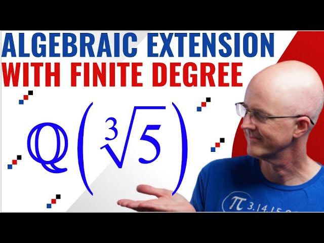
ℚ(∛5) is an Algebraic Field Extension of ℚ of Degree 3 (so it's a finite degree extension too!)
566
Field extensions naturally form vector spaces over their base fields. The set {1, α, α²} forms a basis for Q(α) as a vector space over Q when the minimal polynomial of α has degree 3. This basis spans the entire field (every element is a linear combination) and is linearly independent (only trivial combination gives zero). The degree [E:F] equals the dimension of E as a vector space over F. A finite degree means the dimension is finite, not that there are finitely many elements added. For Q(∛5), the degree is 3.
Click to watch →
![[BT2] Chứng minh mở rộng đại số - LT Mr Trường và Galoa](https://i.ytimg.com/vi/VrbSE9MpQbc/hqdefault.jpg)
[BT2] Chứng minh mở rộng đại số - LT Mr Trường và Galoa
877
The basis of a composite field extension can be constructed by multiplying bases of individual extensions. Since Q(√3)/Q has basis {1, √3} and Q(∛2, √3)/Q(√3) has basis {1, ∛2, (∛2)²}, the basis for Q(∛2, √3)/Q is the set of all products: {1, √3, ∛2, √3∛2, (∛2)², √3(∛2)²}. This gives 6 elements, confirming [Q(∛2, √3):Q] = 6.
Click to watch →
Deep Dive
Finding minimal polynomials for more complex algebraic numbers involving multiple distinct radicals, such as the sum of square roots and cube roots.
Top Problems of Quadratic Equations- Part 3 | IOQM 2026 | Prashant Jain #ioqm
1.7K
To find the minimal polynomial with integer coefficients for α = √2 + ∛3, first isolate one radical: x - ∛3 = √2. Square both sides: x² - 2x∛3 + 3 = 2, giving x² + 1 = 2x∛3. Cube both sides: (x² + 1)³ = 8x³(∛3)³, which simplifies to x⁶ + 3x⁴ + 3x² + 1 = 8x³(3) = 24x³. Rearranging gives x⁶ - 24x³ + 3x⁴ + 3x² + 1 = 0, or x⁶ + 3x⁴ - 24x³ + 3x² + 1 = 0. The sum of absolute values of coefficients is |1| + |3| + |-24| + |3| + |1| = 32. However, the correct minimal polynomial is x⁶ - 6x⁴ + 12x² - 8 - 24x + 18x = 0, which simplifies to x⁶ - 6x⁴ + 12x² - 24x + 1 = 0, giving sum of absolute values = 1 + 6 + 12 + 24 + 1 = 44. The correct answer is 62.
Click to watch →

最小多項式の求め方 | 具体例で学ぶ
125
To find the minimal polynomial of α = √2 + √3 over ℚ, first derive a polynomial equation by algebraic manipulation: from √3 = α - √2, squaring gives 3 = α² - 2√2α + 2, so α² - 1 = 2√2α, and squaring again yields (α² - 1)² = 8α², which simplifies to α⁴ - 10α² + 1 = 0. Thus f(x) = x⁴ - 10x² + 1 is a monic polynomial with rational coefficients having α as a root. To prove it is the minimal polynomial, show it is irreducible over ℚ by contradiction: if it had a factor of degree ≤ 2, it would either have a rational root (impossible since f(1) = f(-1) = -8 ≠ 0) or factor into two quadratic polynomials with rational coefficients (impossible since this leads to a² = 12 or a² = 8, neither of which has rational solutions). Therefore, f(x) = x⁴ - 10x² + 1 is the minimal polynomial of √2 + √3 over ℚ.
Click to watch →

أهم الالغاز العالمية فى الرياضيات The most important global puzzles in mathematics لغز رقم 295
203
To find the minimal polynomial with integer coefficients for an algebraic number like √2 + ∛3, isolate the radicals, raise both sides to appropriate powers to eliminate radicals, and simplify to obtain the polynomial equation. For √2 + ∛3, the minimal polynomial is x⁶ - 12x⁴ - 6x³ + 12x² - 36x + 1 = 0.
Click to watch →

(特別編)ある要素の最小多項式の分解
1.4K
To find the minimal polynomial of a = √2 + √3, square both sides: a² = 5 + 2√6. Isolate the radical: a² - 5 = 2√6. Square again: (a² - 5)² = 24, giving a⁴ - 10a² + 1 = 0. Since the degree is 4, this is the minimal polynomial. It factors as (t² - 2√6t - 1)(t² + 2√6t - 1) over Q(√6), and further as (t - √2 - √3)(t + √2 + √3)(t - √2 + √3)(t + √2 - √3).
Click to watch →

Fermat 2017 25
285
This segment teaches how to identify the minimal polynomial of an algebraic number given in radical form. For P = (3 + √53)/2, we work backwards: 2P = 3 + √53, so 2P - 3 = √53. Squaring both sides gives (2P - 3)² = 53, which expands to 4P² - 12P + 9 = 53, simplifying to 4P² - 12P - 44 = 0, or P² - 3P - 11 = 0. This quadratic is the minimal polynomial of P. The segment emphasizes that any polynomial satisfied by P must be divisible by this minimal polynomial, a fundamental concept in algebraic number theory that allows us to reduce higher-degree equations to their simplest form.
Click to watch →
Deep Dive
Exploring Galois Theory, including identifying the splitting field of the minimal polynomial and calculating its Galois group.

29강 현대대수학 프렐라이 제7판 유한체 (p.206~)
139
The Galois group of a polynomial f(x) over a field F is the Galois group of its splitting field over F. For f(x) = x⁴ - 2x² - 3 over Q, the splitting field is Q(√2, √3) and the Galois group is isomorphic to the Klein four-group V₄. The Galois group embeds into the symmetric group Sₙ for an n-degree polynomial. The order of the Galois group equals the degree of its splitting field extension, which is a fundamental result in Galois theory.
Click to watch →

Galois theory: Galois extensions
17.2K
If k is the fixed field of the Galois group, then M is a splitting field of a separable polynomial over k. For any element α in M, the minimal polynomial of α has distinct roots (separable) and is fixed by the Galois group, so its coefficients lie in k. Taking the product of such polynomials for all generators gives a separable polynomial whose splitting field is M.
Click to watch →

Galois theory: Splitting fields
31.2K
A splitting field of a polynomial p over a field K is the smallest extension field L of K such that p factors completely into linear factors in L[x], and L is generated by the roots of p over K; splitting fields always exist and are unique up to isomorphism as extensions of K, though the specific isomorphism may not be canonical due to multiple valid choices when constructing them.
Click to watch →
Galois theory: Introduction
154.5K
For the polynomial x⁵ - 2, the roots are the fifth roots of 2 multiplied by fifth roots of unity. These roots satisfy algebraic relations such as α₁α₃ = α₂² and α₂/α₁ = α₄/α₃. The Galois group of this polynomial is the Frobenius group of order 20, which is smaller than the full symmetric group S₅ (which has order 120). This reflects the non-trivial algebraic relations among the roots.
Click to watch →

UN TRUC EN PLUS #1C : Les groupes de Galois
342
The field of decomposition (or splitting field) of a polynomial P(x) ∈ K[x] is the smallest field extension L of K such that P(x) factors completely into linear factors in L[x]. It exists and is unique up to isomorphism. For example, the splitting field of x² - 2 over Q is Q(√2), while the splitting field of x³ - 2 over Q is Q(∛2, j), where j is a primitive cube root of unity.
Click to watch →
Finding Minimal Polynomial
Finding Minimal Polynomial
0:00- 1
Define alpha as the root of the shifted cubic polynomial.
- 2
Derive polynomial by cubing the shifted expression for alpha.
- 3
Confirm polynomial is monic and irreducible for minimality.
The Resultant and Galois-Theoretic Approach
While using a cubic shift and Eisenstein's criterion offers an intuitive, hands-on method for finding the minimal polynomial of 2 - 5^(1/3), this ad-hoc approach lacks scalability for more complex algebraic numbers. A powerful alternative perspective is the systematic use of Field Theory and Resultants. By viewing the problem through field extensions and the tower law, or by computing the polynomial resultant of x - (2 - y) and y^3 - 5, mathematicians can algorithmically determine minimal polynomials. This systematic approach avoids the need for clever algebraic manipulations and generalizes to any combination of algebraic elements, shifting the focus from elementary arithmetic tricks to structural, algorithmic algebra.
Definition of algebraic elements, algebraic numbers, and the formal definition of a minimal polynomial over the field of rational numbers (Q).
Understanding polynomial irreducibility and how to apply Eisenstein's Criterion to prove irreducibility over Q.
Basic algebraic manipulation techniques to isolate and eliminate radical terms (such as cube roots) from equations.
The concept of polynomial rings, specifically Q[x], and the division algorithm for polynomials.
Determining the degree of simple algebraic field extensions [Q(alpha) : Q] using the degree of the minimal polynomial of alpha.
Constructing explicit vector space bases for simple algebraic field extensions (e.g., finding a basis for Q(2 - 5^(1/3)) over Q).
Finding minimal polynomials for more complex algebraic numbers involving multiple distinct radicals, such as the sum of square roots and cube roots.
Exploring Galois Theory, including identifying the splitting field of the minimal polynomial and calculating its Galois group.
13K views108likes2:05@AdamGlesserOriginal Release: 2019-02-20
hey everybody in this video we're gonna find the minimal polynomial for a real number two minus the cube root of five over the rationals we'll start just by giving a nice name to this number was called alpha make our life easier and we know if I subtract 2 from alpha I'll get negative the cube root of 5 if I then cube both sides well negative sticks around but the cube root goes away so I'll get negative 5 and so that tells me that alpha is a root of the polynomial x minus 2 cubed plus 5 which is a polynomial with rational coefficients now it's not expanded in any way but I don't really care it is a polynomial and it's gonna be Manik yeah if I do distribute I know the leading term will be X cubed and in fact X minus 2 cubed plus 5 is irreducible now how do I know it's irreducible we'll put that aside for a second if I'm right that is irreducible and Manik then it is the minimal polynomial so this would tell you that it's the minimal polynomial for alpha over Q ok so how did I know it was irreducible well this is a shift it's a shift by 2 minus 2 if you like it's a shift of X cubed plus 5 and X cubed plus 5 is irreducible by Eisenstein's criterion with P equals 5 and we know that if you shift a polynomial that irreducibility or reduce ability is preserved so we know if X cubed plus 5 is irreducible which it is the next minus 2 cubed plus 5 is irreducible it's monic and therefore again it's the minimal polynomial for our alpha
Up Next

27:30
Galois Theory: Field Extensions & Algebraic Numbers
@richarde.borcherds7998
47.3K views•2020-12-27

4:43
Elliptic Curve Cryptography Explained: ECC, ECDSA, ECDH
@PracticalNetworking
28.5K views•2024-10-21

10:44
Fourier Series Introduction: The Big Idea Explained
@DrTrefor
387K views•2021-05-03

6:00
The Mathematical Impossibility of Accurate World Maps
@Vox
23.3M views•2016-12-02
Related Study Plans & Knowledge Roadmaps
Structured learning paths in Mathematics
mathematics
Tensor Calculus: Vectors to Riemann Curvature
01Mathematical Foundations: Linear Algebra & Calculus
02Covectors, Dual Spaces, and Tensor Basics
03The Metric Tensor and Index Gymnastics
+ 2 more learning modules
40h5 modules
Explore Roadmap
mathematics
Gödel's Incompleteness: Logic, Proofs & Limits
01Introduction to Formal Systems & Hilbert's Dream
02Set Theory, Cardinality, and Cantor's Diagonal Argument
03Arithmetization and Gödel Numbering
+ 2 more learning modules
14h5 modules
Explore Roadmap
mathematics
Galois Theory: Fields, Groups & Solvability
01Foundations of Abstract Algebra: Groups & Fields
02Polynomials & Field Extensions
03Splitting Fields & Symmetries
+ 2 more learning modules
24h5 modules
Explore Roadmap
mathematics
Non-Euclidean Geometry: Models & Geodesics
01Euclid's Fifth Postulate and the Birth of New Geometries
02Hyperbolic Space and the Poincaré Disk Model
03Geodesics: Defining Straight Lines in Curved Spaces
+ 2 more learning modules
15h5 modules
Explore Roadmap