
















The Ziegler-Nichols method provides two empirical approaches for determining PID controller gains: the first method uses the step response curve's inflection point to calculate L (distance from origin to tangent) and T (vertical distance), then applies formulas (KP=0.9T/L, KI=1.2T/L, KD=0.075L); the second method involves increasing proportional gain until the system exhibits sustained oscillations at critical gain Kcrit and period Pcrit, then using formulas (KP=0.5Kcrit, KI=1/(1.2Pcrit), KD=0.125Pcrit) to determine controller parameters. Both methods are simple to implement but have limitations and work best for certain transfer functions.
PID Tuning with the Ziegler-Nichols Method: A Tutorial
Added:Understanding the basic components of a PID controller (Proportional, Integral, and Derivative actions) and how they affect system response.
Concept of closed-loop feedback control systems, including error signals, setpoints, and process variables.
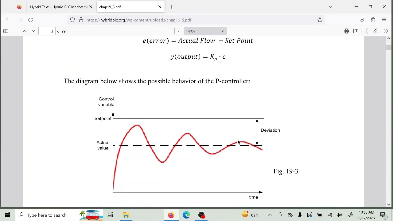
Fundamental knowledge of system stability, including the concept of marginal stability and self-oscillating systems.
Familiarity with transfer functions and transient response characteristics like rise time, settling time, and overshoot.
Exploring the limitations of the Ziegler-Nichols method, such as its tendency to produce highly oscillatory responses, and learning about modifications like the Tyreus-Luyben method.
Studying alternative classical tuning methods, such as the Cohen-Coon method for systems with significant time delay.
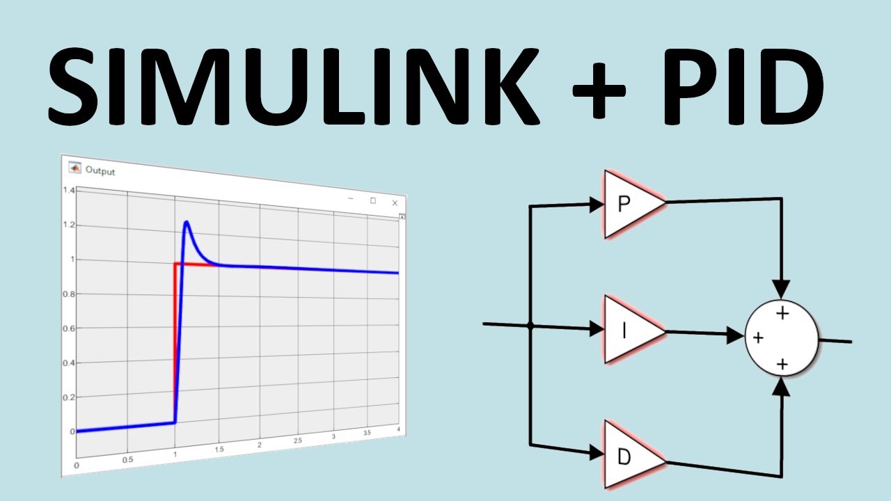
Implementing PID tuning in practical applications using software simulation tools (e.g., MATLAB/Simulink) and physical microcontrollers.
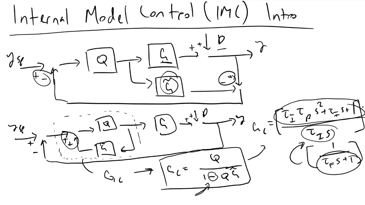
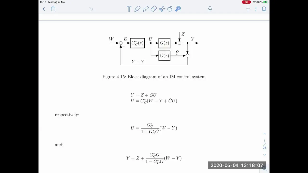
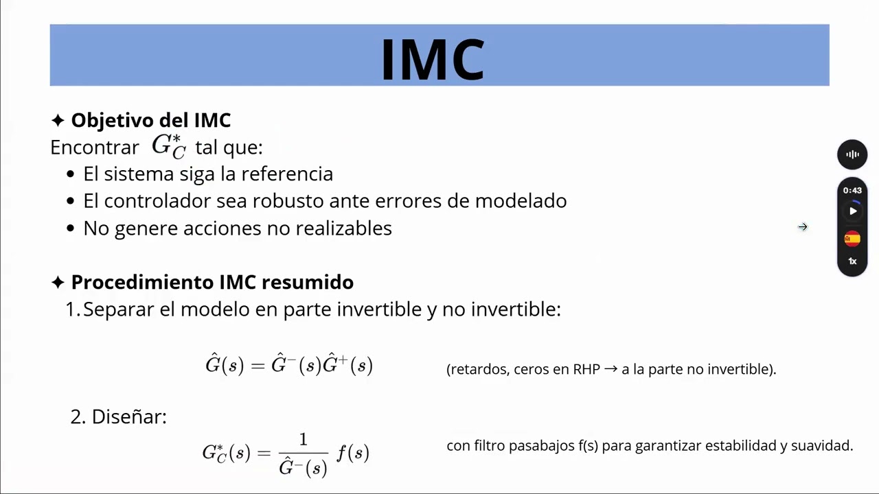
Advancing to modern and robust control techniques, such as Internal Model Control (IMC) or state-space feedback control.
377.6K views2.4Klikes6:19Original Release: 2015-07-11
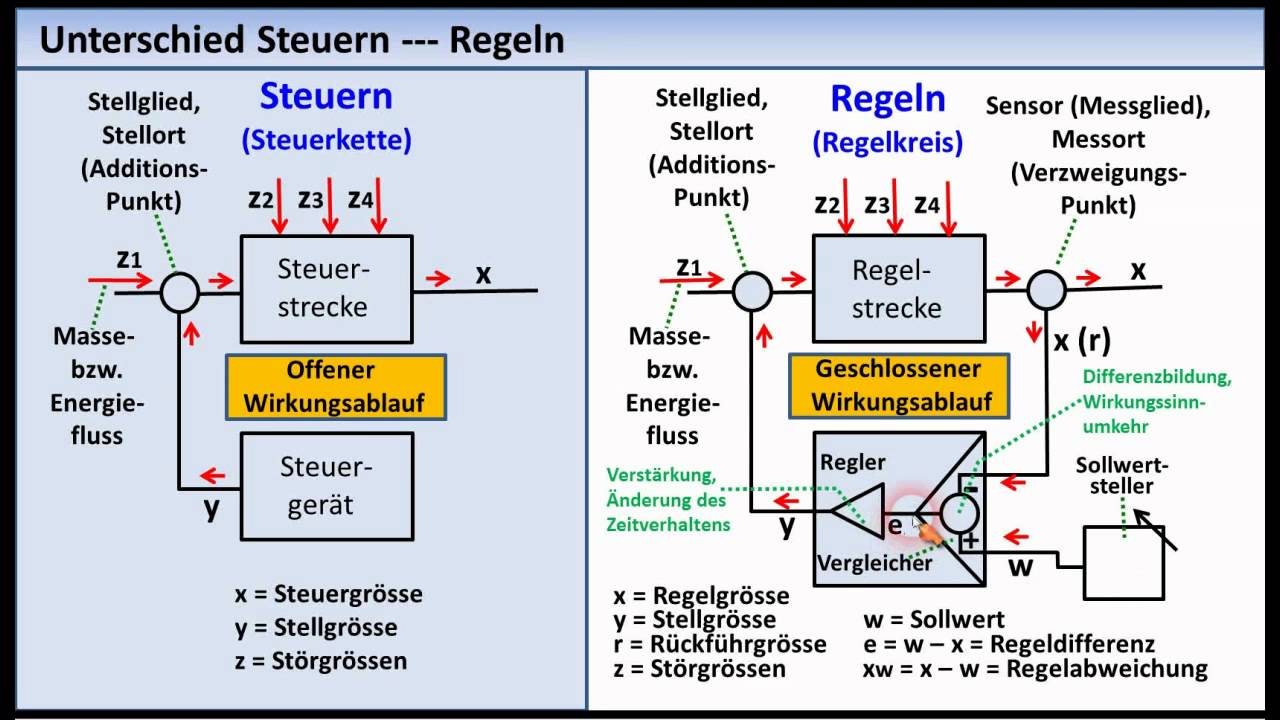
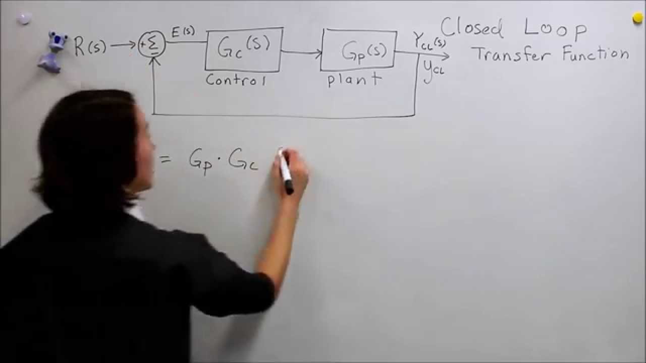
in this video I'm going to explain the Zigler nickels methods of tuning a PID controller this will let you work out what the values of KD your derivative gr gain KP your proportional gr gain and Ki which is your integral gain what Valu should you make these to have a tune system okay so let's look at the first method so for the first method we're going to consider this following system KP 1+ 1/ k i s + KD s so that's your proportion proportional integral and derivative gains and then we've got a plant here and then let's put in some feedback going all the way back here that's minus plus so negative feedback okay so how do we tune this system so how do we determine the values we've got here well let's apply a unit step input and when you do this you'll get a response that looks uh drawing is not very good but let's give this a go a response that looks something like this very rubbish drawing as usual and some value K here so that's when it's leveled off um and you've got some inflection point oh gosh where is it just say say it's here um you can determine that quite easily it's when it changes um so inflection point here is a very important point for determining these um values that you need so draw a tangent to this inflection point something like this and this distance in here from the origin to that um tangent line we're going to call this distance L and then if we come from where this line here which comes along from this steady state intersects with a tangent line drop a vertical line down there and from this point to this point we can call this distance T and we can make up a table from this of what values we should have so we've got a proportional controller proportional and integral controller and then a p controller and then you've got values KP Ki and KD um so that should be T / by L you can determine these by now you've got enough mathematics to easily determine these um 0.9 T over L 1.2 T over L this one is infinity of course that's zero this is of course zero because you've got no D here um this should be L over 0. three this should be 2 L and this should be 0.5 l so use this table once you've got your T and your L and you get all of the values that you need okay let's move on to the second method the second method is very very easy it's very nice basically set up this system so we've got block there KP then we've got a plant plant here and then some feedback just shooting around all right now how do we determine the values that we need for our P ID controller so let's put um Ki and set that to Infinity let's set KD equal to zero so that's kind of the system here if you look at the previous um system we had you'd end up with that when you applied this okay so we want to determine this thing that we're going to call K crit or k critical this is the point at which the system becomes marginally stable so you get a little bit of oscillation so you increase in KP to um go okay can spell increase KP P2 K crit and you'll get a response that looks something like this at k equal K crit something like this it's just started to be unstable and you get this thing here P crit and this is KP equals K crit this is a critical okay very simple just simulate this system increasing KP until it becomes marginally stable so it's just first exhibiting sustained oscillations something like this and we have the value K crit and we have this value P crit and then we can just get this table P Pi I and then p i d so KP is 0.5 * K crit in this case we've got KD here sorry Ki just we have written my table I'm copying from so infinity and then zero of course no D zero here no D um 1 over 1.2 P crit here you've got 0.45 K crit uh 0.6 P crit 0.5 P crit and then 0.125 P crit okay so that's your two methods very quick overview both of them are extremely simple simple very convenient to use um it has its limitations it's not a perfect method and can only be used in certain circumstances um for certain transfer functions um hopefully this is useful to you and you can now do it it is really simple to do and thank you very much for watching
Up Next
17:33
Understanding Digital Audio through the Nyquist-Shannon Sampling Theorem
@TechnologyConnections
583K views•2018-08-10

30:32
Ultrasonic Transducers: Resonant Frequency Measurement and Horn Design
@imajeenyus42
229.9K views•2017-02-22

54:16
Polymer Environmental Degradation: Mechanisms & Stabilization
@iit
1.8K views•2012-07-10

33:39
How a Student's Question Saved a NYC Skyscraper from Collapse
@veritasium
22.8M views•2025-04-26
Related Study Plans & Knowledge Roadmaps
Structured learning paths in Engineering
engineering
Building Acoustic Levitators: Physics & Arduino
01The Physics of Sound and Standing Waves
02Piezoelectric Transducers and H-Bridge Drivers
03Arduino Programming: Generating 40 kHz Signals
+ 2 more learning modules
14h5 modules
Explore Roadmap
engineering
Building Peltier Cloud Chambers: Particle Tracks
01Cosmic Rays & Cloud Chamber Physics
02Thermoelectric Cooling (TEC) Fundamentals
03Custom Liquid-Cooling Loop Design
+ 2 more learning modules
18h5 modules
Explore Roadmap
engineering
Yagi-Uda Antennas: Modeling, Build & VNA Test
01Introduction to RF and Antenna Fundamentals
02Yagi-Uda Antenna Design Principles
03Antenna Modeling and Simulation in 4NEC2
+ 2 more learning modules
18h5 modules
Explore Roadmap
engineering
ECG Monitor Design: Op-Amps, Filters & Noise
01Electronics & Breadboard Basics
02Op-Amps and Instrumentation Amplifiers
03Bioelectricity and ECG Fundamentals
+ 2 more learning modules
18h5 modules
Explore Roadmap