





![[Hindi] Python Matplotlib Tutorial - Python Data Science and Big Data Tutorials](https://i.ytimg.com/vi_webp/VFsRLjSc8GA/maxresdefault.webp)



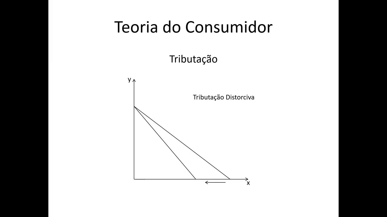


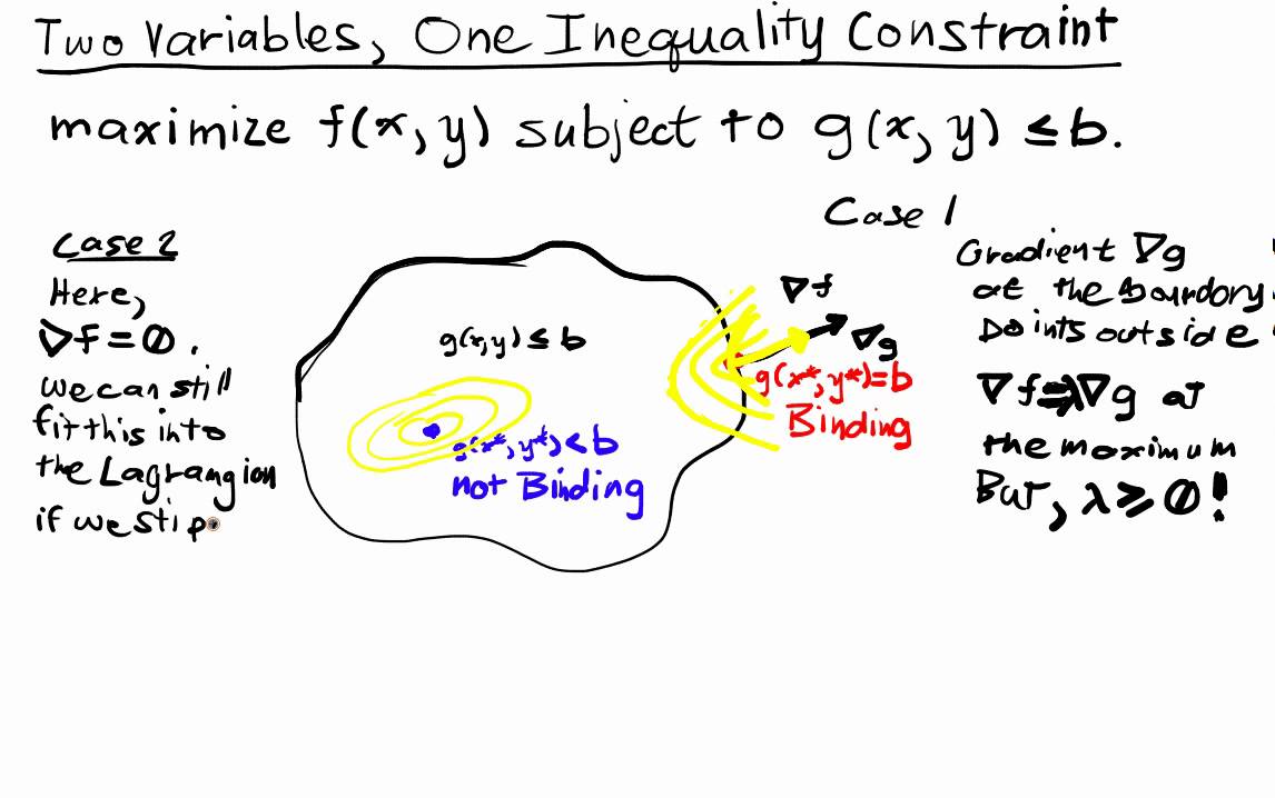














In a labor supply model with progressive taxation, consumers maximize utility by choosing consumption and labor supply, where consumption provides positive utility and labor supply reduces it. The model includes a standard labor income tax and a top bracket tax on income above a cutoff. Numerical optimization reveals that labor supply generally increases with wages but decreases at the top bracket cutoff, as workers reduce labor to avoid higher marginal tax rates. This demonstrates how progressive taxation creates a trade-off between tax revenue and labor supply incentives, with optimal tax rates balancing revenue collection against economic efficiency.
Labor Supply Choice and Taxation: Numerical Analysis for Economists
Added:The microeconomic model of consumer choice, specifically the labor-leisure trade-off and utility maximization under a budget constraint.
Basic Python programming skills, including the use of libraries such as NumPy for numerical operations and Matplotlib for plotting and visualization.
Fundamentals of taxation, including how marginal tax rates alter budget constraints and consumer incentives.
Introductory calculus and optimization techniques, particularly first-order conditions and constrained optimization.
Exploring the Laffer Curve numerically by simulating how aggregate tax revenue changes across a full range of tax rates.
Analyzing non-linear and progressive tax systems, which introduce non-convex budget constraints and require advanced numerical solvers (like SciPy's minimize).
Studying optimal taxation theories, such as the Mirrlees framework, to mathematically balance economic efficiency and redistributive equity.
Extending the static labor supply model to dynamic, multi-period frameworks, such as lifecycle models of savings and retirement.
406 views1likes18:07Original Release: 2023-03-06
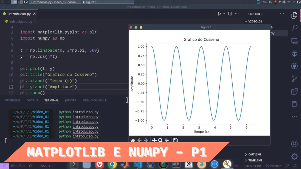
welcome to today's video on labor Supply and Taxation in this video we consider a consumer solving the following maximization problem where the consumer has to choose how much to consume and how much labor to supply uh consumption is good that gives you utility labor Supply is bad that decreases your utility what you can consume is whatever you got in resources X and your resources X is the sum of your cash in hand to begin with the wage income you get from supplying a labor so that's the weights times labor Supply minus your taxes where the taxes is a standard labor income tax which just multiplied the the total gross wage income and then an extra tax which is an all labor income above a cutoff copper so that is so this is a a top bracket labor income tax labor supply has to be between between 0 and 1. analytically this is a bit irritating to solve this problem because of this this this maximum here which implies that it's not differentiable uh so it's a good sort of example of why where it's it's easy to use on a Miracle Solution instead one thing we can realize about the problem is that because the utility is monotonically increasing in consumption so that is you can always get more utility if you consume more then you will always choose to consume all of your resources so more no matter your decision and labor Supply we know that your consumption Supply is just to consume everything the Baseline parameters that we will be considering is that is the um uh is that the initial resources or the level the cash in hand is is one the utility effects on on labor Supply is this new is 10 the the Epsilon here which will which is can also be called the fridge elasticity of label Supply is point three the standard labor income tax is point four the top bracket income tax is 0.1 and the cutoff is is 0.4 now the questions in this is that you should construct a function which solves the consumer problem giving these parameters you should plot the the optimal Choice functions as functions of of the wage in the range 0.5 to 1.5 then you should consider a population with 10 000 individuals indexed by I where you should assume that the distribution of weightage is uniform such that the wage of the ith individual is drawn from a uniform distribution between 0.5 and 1.5 and we denote the optimal choices of eating the individual by L star I and C star I for the labor Supply choice and the consumption choice and then the final question is to calculate the total a labor tax revenue by simply summing up over all individuals so this is a good time for you to pause the video and try to provide a sketch on how you would solve these these three problems it will take some time for you if you actually wrote up the code but it's a good idea to sort of to have a sketch on on what are sort of the steps that you will have have to take and then you will sort of be better able to to follow the the way I suggest to do it if you have thought about that beforehand so let's go to the solutions so the solutions uh uh in this notebook and then they are in this labor supply model dot Pi this five which will contain some functions that we will be loading we will return to that in a minute you can see that the file is over here in the editor so it's so it's it's readily available I import numpy and I import matplotlib with some settings and I use the auto reload magic when I before I import the label supply model as LSM uh because then if I made changes then they're sort of updated when I run in the notebook so let's let's run this and that's that's now done then I Define all the parameters uh exactly as as I roll over above so there's nothing special in that I just want this this line then the first thing sort of more technically I need to do is I need to allocate some space for my Solutions so I know I will have a thousand individuals and I will just do a vector of the wages between 0.5 and and 1.5 of the Thousand individuals and I've used this lid space function in numpy which is exactly sort of return evenly space numbers over specified interval and then for the labor Supply choice in the consumption choice I will just use uh zeros in here so let's that let's run that now we're actually ready to uh to find the solutions so what I what I do is I Loop over all individuals and then I call this find Optimal labor Supply function which is in this uh LSM module and that provides me with the solution for labor Supply and given this I also get a uh an implied consumption choice so I'm going to just run this and I have solved it but now of course we need to understand this code a good trick is you can always place your your cursor on on the function and then you can press F12 to go to the function definition so let's do that and now it opens up you can see that it opened up this this file and it went directly to this uh to this to the to this function here uh it's always a good idea I think when you come to a function like this to to understand sort of what does it do and the first thing you can do sort of is look inside the function it describes what the function is doing that's very clearly stated from the name and then it describes each of the parameters and telling you what does these parameters what should they these parameters be what should these arguments be and then it says okay what does it return it would turn the optimal label Supply and you can understand so what how how is this done you can see it's doing that by creating a Lambda function an objective which is a function only of the label Supply and it takes in minus the value of choice given this label Supply choice and the parameters and then it's using from the uh from optimize which is a module from from scipy it's using the minimize scalar which is a way to minimize a scalar function so it takes this in this function now which is only a function of the label Supply and it optimizes minimizes this so we that's why we have the negative in in front here um and doing that within the bounds from zero to one uh because I'm and I'm using the method called call bounded here so in that sense it's easy to understand what this is doing but there's two things that are hard here one thing is what is this value of choice function doing we need to dig into that and to some degree it might also be hard to understand the minimize scale up but you could you can take that as as a black box to some degree and now this is some somebody else would have written that that code and that just just works and you can see once we get the result out from the from the optimizer then we return the x value in in the result which is actually the just the optimal labels but once you sort of understand what's happening inside a function it's good to have an overview of the whole module so it's a good thing to collapse everything such that all the functions in here are collapsed then you can see okay what's imported very important in numpy and we're importing the the optimized from sci-fi and then there are a number of functions that are defined here we always saw the value of choice function and we can see that there's also a utility function which takes the inputs of both consumption level Supply and some parameters and probably calculate utility we can see here that is utility of consumption labor Supply decisions that make sense uh we can also see that it's a way that once we have the uh the label Supply we know the implied C so we can calculate that so we have a function for that and when we load Level side we also have to imply text so we can calculate uh calculate that so let's try to dig into this so what's happening in the value of Labor Supply a value of choice sorry um you can see that it's actually using the implied C function to calculate consumption and end it returning the utility value from the consumption in the label supply chain and of course it's always given all these parameters so if we do dig into that then we can see the utility that's just the formula for the utility that we had in the notebook the lock of consumption minus the new times this expression for the test utility of Labor and then we have the implied C which is basically just a calculation of of the X the cash in hand plus the wage income minus taxes which now uses the implied taxes function so we can go into that which is the formulation of of the tax system from The Notebook the base tax times the labor income plus the uh the the tax on the top bracket of Labor income Above This cutoff cover so in this way we have now take through all of these functions and sort of have an idea of what they are doing if this went a bit too quick for you just pause the video and try to look at these functions yourself and see how they are calling each other and and and the uh and what they're they're doing so you'll have an overview of that but let's return to the notebook device so we have called the function so we have found the the solutions but one thing that's a good thing to think about here is what about the order of the arguments it's clear that we need all the arguments to find the optimal choice because they they all if the effect the the the choice in one way or another but why in this exact order could this order be different or would that be a problem uh try to think about that for for a minute so we could not change this all around right if we will get the wrong result if I changed around this that would just be wrong because now the the the function in here would getting getting the wrong argument so I would use Taiwan for Tau 0 and Tau 0 for Tau one so that just doesn't doesn't work so it's important to keep the right order of the arguments that's in general shows it's a problem with long list of arguments because you can easily make mistakes in that um so that should be avoided if we can so this is something that's a bit bad about the implementation here it's very simple because it just States all the parameters and then puts them in but it means that we have to have the right order of these things we cannot mess that up one thing that sort of helps by doing that is to keep the the aura the same so we can see here that this order is exactly the same as the order that we have down here so sort of sort of keeping the order fixed helps by that but sometimes you will still mess it up so really be aware of this but okay let's have a look at the results so we had to plot uh the label Supply and the consumption charge against the the wages so let's uh to to do that and this is exactly the what what we get out you can see that the labor Supply is generally increasing in in the weight you want to to work more if if the wage is higher except in this interval here where we can see that actually label Supply is decreasing when the weight is increasing and if we look over to the consumption charge you can see that's a point where the consumption is is exactly flat uh so you can show if they got it a bit more into this as this is because this is exactly at the cutoff you don't want to sort of increase your level Supply uh when your wage increases because then you would get to pay the the the the top tax and you want to avoid wipe that so just reduce your labor Supply to keep your your labor income uh constant and therefore your consumption will always all also be big constant so this shows it's rather easy to get such a result out of our numerical solution which will take a bit more sort of uh work if you wanted to show something similar uh in in analytical terms okay for the final question we needed to calculate the the tax revenue and a smart small trick we can use is that we we can use that an equally spaced Vector approximately the uniform distribution so if you haven't equally spaced uh Vector then it's exactly like we're just putting out the 1000 individuals between the the lowest and the highest wage point which is exactly how uniform distribution looks like so we can actually just take the sum of the implied tax of the optimal labor supply for the wages and then we can yeah sum that up and then we get the total tax revenue and this looks like this we could also have used random sampling so we could have said okay let's show set some seeds so that we can reproduce the the results let us run 50 replications because now the result will change for each each draw let's save a vector of the total tax revenues uh of each repetition let's go through the repetitions each time we draw our new distribution of wages we use the uniform distribution between 0.5 and 1.5 we set in a thousand individuals the N here then we allocate some space for finding the optional level Supply and we call this find Optimal level function for this value of of the wage then we find the tax revenue just as we did before by by summing up across individuals and then we print the tax revenue if for the first 10 repetitions and for each 10th reputation after that and finally we will plot the mean and we'll probably plot the minimum and the maximum value so let's let's try that you can see we get something that is in the ballpark of what we got up here it takes a bit longer uh and instead of it jumps a bit up and down just wait for it to finish um I said in 50 so now it's finishing and it gets something that's close to but not exactly and you can see that it has some some span up here so it's good that they give approximately the same results if we increase the number of reputations we'll probably get something that's that that's very similar uh but this of course up here was much faster and didn't need sort of any of the problems with rehabilitations and so on but it's always good to think about different ways to solve the problem and show that they get you at these approximately the same result that make you more confident that your factory found the right solution okay finally uh sort of an open question to end this notebook what determines the tax revenue um you should spend some time trying to change parameters change Tech parameters preference performances energy resources maybe change utility function maybe change the distribution of wages for example uh to unlock normal or or a a operator and see how does that affect the tax revenue that that's a good way to get into Asian for how this this model works let me just show you one thing that might be interesting we can't say okay what what would happen in this model if we increased uh the top income tax uh so let's start with what we had in point one and then let's just increase it to uh to various uh higher levels up here and now let's say okay we want to to do basically the same thing as we did before so we can use the code that we had so we can copy in our code for the optimal label Supply here this and we can copy in our line for the total tax revenue and we also plug in what we have for the printing so that's fine now I also want to remember what the the top isolated let me instead do it like this okay so let's see if everything right and now we can oh I did something wrong I write it out it's like type one instead so now we can see that okay we start by uh by this text menu and actually we get a smaller tax revenue if we increase child one so that was sort of interesting could we perhaps get a larger tax revenue if we decreased it we could actually get a slightly larger tax revenue but if we go very low then then the tax revenue is is is is falling again so there's a lot of limits here on on on how big we can get the the tax revenue uh of course that will change with the other preference parameters and the distribution of wages and so on so that's something that could be interesting to investigate thank you for today
Up Next

68:27
Understanding Taxes: Economic Impact & Policy Trade-offs
@MercatusCenter
3.5K views•2010-11-08

5:07
Impact of Yuan in Indo-Russian Trade Amid Sanctions
@WION
261.9K views•2022-07-01
10:33
Behavioral Economics Explained: Rationality, Nudges, and Risk
@crashcourse
1.1M views•2016-03-12

113:18
The Age of Easy Money: Fed & Inflation | Full Documentary
@frontline
21.2M views•2023-03-15
Related Study Plans & Knowledge Roadmaps
Structured learning paths in Economics
economics
Sovereign Debt: Defaults, IMF & Restructuring
01Introduction to Sovereign Debt & Government Bonds
02Debt Sustainability & Credit Ratings
03Anatomy and History of Debt Crises
+ 2 more learning modules
12h5 modules
Explore Roadmap
economics
Market Design: Matching Theory & Gale-Shapley
01Introduction to Market Design and Price-Free Markets
02Two-Sided Matching & The Gale-Shapley Algorithm
03School Choice Systems and Mechanism Design
+ 2 more learning modules
10h5 modules
Explore Roadmap
economics
Impossible Trinity: Forex, Capital & Policy
01Introduction to Monetary Policy and Central Banking
02Exchange Rates and International Capital Flows
03The Mundell-Fleming Model
+ 2 more learning modules
8h5 modules
Explore Roadmap
economics
Healthcare Economics: Market Failures & Systems
01Introduction to Healthcare Markets and Market Failure
02Asymmetric Information and Adverse Selection
03Moral Hazard and Insurance Design
+ 2 more learning modules
12h5 modules
Explore Roadmap