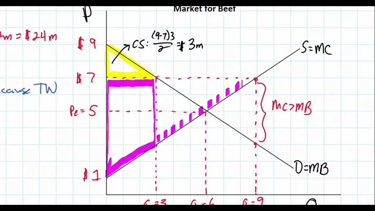
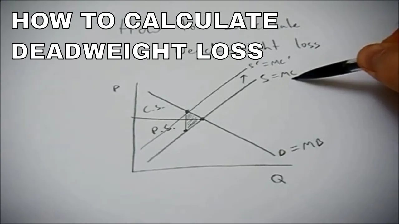
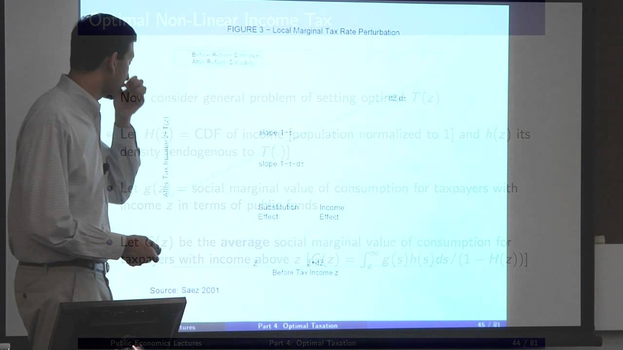
Optimal Taxation Theory: Ramsey Rule | Economics Lecture 1

[00:00:00]I'm going to talk about the next section of the class optimal taxation all right so we're going to talk about four uh sets of things we're first going to start by talking about commodity Taxation and the classic Ramsey rule one of the most important results in optimal tax Theory then we'll talk about capital income taxation and spend a particular amount of time on the retirement savings literature which fits into it's like an empirical analog to the type of stuff we'll talk talk about here and is very active right now uh we'll then talk about income taxes and the Merle's model and focus in particular on implementing the Merle's model empirically uh drawing on the work of manual sias and others and then we'll talk about optimal transfer programs like the optimal design of the eitc or uh trans other transfers in kind transfers to low-income people and so forth so the way you want to think about optimal commodity taxes is that we're essentially going to combine the lesson we've learned on the incidence and efficiency costs of taxes to now ask the normative question of what's the best tax system given some objective function right and what is that objective function going to embody typically equity and efficiency concerns right we're concerned about the size of the pi and we're concerned about how the pi is distributed and we're going to build both of those in to say something about the optimal system so from a purely efficiency uh point of view the problem is really simple we would Finance the government purely through lumpsum taxation right we know that lumpsum taxes don't distort prices don't generate dead weight loss and so we should just use lumpsum taxes but once you have redistributional concerns this becomes much harder because ideally what you would do when you have redistributional concerns is Levy individual specific lumpsum taxes so what why do we care about redistribution what in the Mer's model it's that some people have more skills than others okay so some people uh let's say end up in the most extreme case having a disability or end up you know having a lower ability to generate earnings than others if I knew Exane who those different people were what I'd want to ideally do is just Levy a head tax on each person you know I see like suppose to take the example we talked about before height is the only determinant of earnings I would just Levy a height specific income tax right uh and not condition it on wages at all in practice we we don't have such good predictors of who who High ability and whose low ability and so we end up being forced to redistribute on the basis of expost outcomes so you made a lot of money you must have been high ability I'm going to tax you a lot that ends up being a distortionary tax because it distorts your incentive to work hard uh and that creates the trade-off between equity and efficiency right so uh you know whatever outcome you're taxing income or consumption you're going to end up with these distortions and so that's going to motivate the types of policies we're going to study so so at a high level it's very useful to keep in mind that there are two broad approaches to Optimal taxation one is called the Ramsey tradition which I think of as essentially restricting attention to linear tax systems so think of t.x type of tax systems the and then there's the merian approach where Merle says you know why do we restrict ourselves to this particular tax instrument let's allow for nonlinear tax systems where it's t ofx with no restrictions on T ofx and in particular importantly I'm also going to allow lumpsum taxes right so in the Ramsey approach I'm going to rule out the possibility of lumpsum taxes by assumption and consider linear taxes so I'm going to say there are reasons which I'm not going to model that I don't want to use lumpam taxation so let's restrict attention to distortionary linear taxes and solve for the optimal policy merly says uh let's not make any adhoc assumptions about what is or is not permitted in the tax system let's permit you to implement lumpam taxes but let's model their costs their endogenous costs uh in a model with heterogen right so if I impose too much lumpsum taxation in the merian model that's going to end up being undesirable because it takes too much money away from low-income people relative to high income people and so I'm going to allow the lumpsum tax and then solve for the optimal tax system uh directly so we'll uh pick up there next time and so naturally you would think you want to tax things that are more elastic less and will derive that optimal Ramsey tax formula in this lecture the second uh very influential and famous set of results is due to or due to shamley and Jud in two separate papers uh which show that it's optimal to have zero capital income taxes in the long run in infinite Horizon Ramsey models and we'll also touch upon that uh in this lecture and we'll talk about how this result has actually shaped the policy debate quite a bit because that's kind of behind the scenes and why many people think we should have low capital income tax rates relative to labor income tax rates but has been challenged in more recent work the third result is uh due to Diamond and Merle's which is a result that's called production efficiency we will not cover that in this class but just so you're familiar with what it is uh it's the idea that you always no matter what your tax system is you want to maintain efficient production that is you want to be on the frontier of the production possibilities uh Set uh and so as an example of the kinds of things that rules out you don't want to tax intermediate inputs is one prediction of their theorem they show under very general conditions no matter what tax instruments you're using you want to produce efficiently which kind of makes sense why do you introduce unnecessary distortions into the production process when you could just tax the final goods anyway and that's the logic of their result uh and then the fourth result which I'll briefly describe here but you'll cover in much more detail because there's a literature surrounding it is the Atkinson and stiglets result which combines the merian model of optimal progressive income taxation with the Ramsey type models we're going to talk about here where we have linear taxes on Commodities and their result is that if you have access to a progressive income tax you don't need to use consumption taxes at all that is you can achieve the uh um second best optimum the best you'll ever do given the information constraints just using the progressive income tax another way to State this result is that consumption taxation is Superfluous and the reason that connects that actually connects to this sham and Jud result because as we'll talk about later you can think about taxes on savings as basically taxes on consumption Goods where the two consumption goods are two different periods right C1 and C2 and so this result is another rationale for why you might not want to tax capital income and we'll talk a little bit about that later on so just keep in mind at the broadest level these are four uh important results and then we're going to go into the mathematical detail of each of these things but I don't want you to lose sight of the big picture okay so we start with the Ramsey uh tax problem which is the simplest and classic optimal tax model so in this model the government sets taxes on uses of income say consumption Goods in order to accomplish two objectives the government wants to raise a total amount of Revenue of e which we're going to take as exogenous so you want to build a bridge that costs a million dollars or something and you want to you're benevolent social planner so you want to raise that tax in the most efficient possible way in particular um maximizing the agent's utility uh subject to this Revenue requirement or minimizing the utility loss due to the tax so there are three critical assumptions in the Ramsey model first we prohibit lump suum taxation okay so remember I talked about in the end of the previous lecture the distinction between the Ramsey and the meres approach in the merian approach you permit whatever taxes you want to implement in the Ramsey approach you uh you eliminate lump suum taxation because if you allowed lump suum taxation we know the answer to this problem is Trivial if you want to finance e dolls of a public good you would just Implement a e doll lumsum tax right that's going to create no distortions and be the most efficient way to raise the revenue but that's not an interesting problem we think that in practice for reasons related to redistribution which we're not modeling here we can't we're not actually going to want to use Lum some taxes and so we just rulle that out by assumption uh in the Ramsey approach second we assume that we cannot tax all Commodities that is there's at least one commodity that we cannot tax so can somebody say why this is why is that assumption important so so what happens if you can tax every consumption good or tax consumption and Leisure yeah it's equivalent to a lumpsum tax right if you can tax everything you don't end up distorting relative prices right uh and so as a result there's uh effectively you know you effectively have access to a lumpsum tax so one way to think about it is there's no way to tax Leisure uh you know typically leisures uh untaxed so that's why you're changing the relative price of consumption goods and and Leisure say with an income tax or taxes on consumption uh and so you know we think that this is also a reasonable assumption and is analogous to number one the third assumption we're going to make uh which is not critical to the Ramsey approach but is uh you know standard when analyzing these types of models is that we assume producer prices are fixed okay so constant uh uh sorry infinitely elastic Supply curves so you know producers are not going to bear any of the incidents of the tax and then just as a normalization this is not an assumption just normalize all the pre-tax prices to one because it it's not going to affect anything and so I'm going to denote by Qi the post tax price of good ey which is going to be 1 plus ta I where taii is the specific uh tax on good ey okay so we have one individual in the Ramsey model uh and so you know we have no explicit redistributive concerns right so I just want to be clear um someone asked me a question after lecture which is also relevant to the efficiency analysis uh which is why do we assume the the way we're going to think about this problem is the individual does not internalize the effect of uh his behavior on the government budget which might seem like a weird assumption in the context of a model where there's only one agent but the way we're thinking about this is that in uh in the broader economy if you're thinking about your own choice of how much to consume of a good you're not going to take the feedback effect onto the government into account right that so what's the feedback effect in this model if I change my behavior I reduce consumption of good eye because you have a higher tax on it if I literally benefit from the public good that you are supplying then you might think okay with a single person I take that into account because there's a one forone effect on the government budget but we're going to assume that you optimize ignoring the fact that the government budget's going to change when you change your behavior what are we trying to capture in an economy with a million agents your own impact that you know if you consume more candy bars that has a trivial effect on the government budget so to first order you uh ignore its impact on the government budget and take it as fixed right so just think of this so we make this assumption here as we did in the efficiency analysis we don't internalize the impact on the government budget that's that's an approximation of what would happen if if you had a lot of Agents right any one agent has little impact on the provision of the public good okay so given that assumption the individual maximizes his utility function over the N goods and say uh labor L to satisfy this budget constraint so this is his uh expenditure on the left hand side and then total income on the right hand side where notice I don't allow a tax on L right okay so we first uh describe how we solve solve the individual's problem and then we'll think about the government's uh problem so the lran for the individual's maximization problem is standard so this is his objective the utility function and then this is his budget constraint we're going to let Alpha denote the multiplier on the budget constraint and you get the standard first order condition that you set the marginal utility of consumption of good ey equal to Alpha the multiplier on the budget constraint time Qi the price of good ey okay so Alpha which is equal to DV DZ the marginal utility of an extra dollar uh represents the marginal value of money for the individual all right that's the interpretation of that multiplier uh in this standard utility maximization problem so that problem is going to give you demand functions XI of Q comma Z so demand for each good marcelian demand functions and an indirect utility function B of qz where Q just to be clear denotes the entire price Vector including the wage rate W the government uh now solves the maximization problem Max V of qz so the government is maximizing the agent's indirect utility so here you see the standard setup of optimal policy problems in Public Finance where you have an individual problem where the individual is choosing Behavior to maximize his own utility and then the government problem nests the individual's problem where the government is setting the taxes to maximize the individual's indirect utility or value function where the value function is a function of the choices that the individual makes subject to some Revenue requirement or some B balance budget constraint for the government right so the government's Revenue requirement is just that t.x the total amount of Revenue it collects has to be greater than or equal to e notice that in the government's Revenue requirement enters the individual choices right the the qis CH the XIs chosen by the individual are going to affect the amount of Revenue the government generates and that's going to be the source of the Dead weight loss and the uh inefficiency that matters for optimal taxation now you can equivalently write this problem with its dual which is to minimize the excess burden of the tax system so you can say the government if you remember just think back to our definitions of excess burden uh EV valuated using the expenditure function for the individual minus the revenue requirement uh you can equivalently think of the government is trying to minimize excess burden subject to raising that same amount of Revenue and we won't do this here but you'll see you can show that you get exactly the same formulas if you solve that second problem instead of the first okay so let's start to think about how to solve this so first we're just going to do it uh algebraically and then we'll talk about the intuition so for the government's maximization problem the lran is again given by the objective plus Lambda times the constraint Lambda now denotes the multiplier on the government budget constraint right so let's differentiate that with respect to Qi equivalently it's the same thing as differentiating with respect to TA the tax on good ey so what comp components does that have so you have a DV dqi that represents the private welfare loss to the individual raising the price of good ey then you have this mechanical effect on Revenue which is if I raise taii by a dollar the mechanical Revenue that I get get is proportional to XI the amount that guy was spending on that good and then you lose some revenue from the fact that when you raise the tax there are going to be changes in behavior and changes in Behavior not just in the consumption of that good but consumption of all potential goods and if you have tax on all the goods then that's going to affect your budget constraint through all these terms here okay so now to uh go further we're going to use Roy's identity which tells us that the marginal uh impact on utility of raising the price of good ey is just minus Alpha * XI okay so how do we interpret that Alpha is the marginal uh value of money right the marginal utility of a dollar and excise the amount you're spending on good ey this is just an application of the envelope theorem right if I if you're spending 10 if you're buying 10 units of a good and I increase the price by a dollar your utility loss is equivalent to the marginal value of $10 to you because we don't need to worry about the fact that you're going to reoptimize your consumption because that has a second order effect right so the the Lost uh value is essentially what is $10 worth to you and Alpha tells you what $10 is worth to you right so Alpha times the consumption of the good the government uh okay so so we get minus Alpha XI here right okay so now we let's combine terms so we get a Lambda XI minus Alpha XI that's the first term here and then we get the second term that's coming from the behavioral responses so notice that the difference between Lambda and Alpha measures the marginal value of a dollar to the government relative to the individual okay and so what's the way to think about that the government uh might value money more than the individual if these public goods have a benefit right the government's actually doing something useful with the money notice that we get a direct connection to the marginal excess burden formula where Lambda equals Alpha right so the way we were thinking about excess burden before there were no benefits to the government doing any taxation so you can just think about that as the case where Lambda equals Alpha and Lambda equal 1 uh and so that first term drops out and all you get is the second term which you'll recognize as being similar to the excess burden formulas in fact it's the same thing it's the revenue leakage version of these formulas that's exactly what it is okay so then just carrying through with the algebra you can see that the optimal tax rates are going to satisfy a system of n equations and N unknowns which look like this they depend upon these uh price elasticities and then they depend upon intuitively just the relative value of money for the government relative to the individual okay so now we're going to rederive that formula using a technique that I think is very useful in a lot of applications which is a perturbation argument it's useful to get intuition on what matters for optimal policy and what the key forces are in determining uh optimal tax rates or optimal social insurance or any number of problems that we're going to talk about so the idea of the perturbation argument is really simple you say suppos I'm at a given tax system right we know that if I'm at an Optimum a necessary condition is if I perturb that system by a little bit it should have no impact on welfare now that's not in general a sufficient Condition it's a it's uh you know it requires concavity right so the it requires Global concavity if that's uh the case then we know that if the first order condition is satisfied uh you're at the optimum but you know at the least that this is a necessary condition if you can perturb the tax system by dii and gain welfare you can't possibly be adopted right okay so suppose the government increases T from some level uh by Dai by some small amount what is the effect of that tax increase on social welfare well it's the there're basically two components there the there's the effect on private Surplus the utilities of the agents and the economy in this case and there's the effect on government revenue right so what's the effect on government revenue let's start with that so these are the terms we had before if I raise the tax rate by Dai I gain extra Revenue through the mechanical effect of just XI * dii and then I have these behavioral responses where dxj denotes the amount that I change consumption of XJ when I have this perturbation okay and so I'm going to gain or lose revenue on these Dr Goods depending upon the DX for all of those goods what's the marginal effect on private it Surplus that let's call that du that's given by DV dqi so what does the guy lose when you raise uh the tax rate by $1 times the amount you change the tax rate dii on that good right and so what you get is uh here just again applying gr's identities minus Alpha I Alpha XI d right so the idea of the perturbation argument is that at the optimum uh this perturbation should have zero impact on total welfare and so we we basically if we add the two effects and we put this weight Lambda on government revenue so that's the value of government revenue relative to individual consumption then we have to have du plus Lambda Dr equals z which uh exactly gets us back to the formula we had before if you just look at the previous page the sum of those terms is exactly what we derived just by directly differentiating that equation okay so it's intuitive that you're basically setting the marginal gains from another way to think about it if I just come back here this is the marginal value of raising the tax in terms of uh the wedge between Lambda and Alpha that's the extra benefit you're getting from that government expenditure and this can be thought of as the efficiency cost that you're incurring and so you set those two equal uh at the optimum so that they balance out okay any questions on the basic setup yeah all because so the government let's say is taxing apples and bananas right so if I change the tax on apples it's going to make you buy uh fewer apples let's say if I increase it uh but more bananas and so I need to if I I need to look at total government revenue right to look at the impact on the budget so I need to take into account the impacts on all the other markets as well right questions okay so now we're going to rewrite this formula in a few ways and talk about its properties okay so the first thing that people often do um is rewrite the formula in terms of hickie and elasticities in order to obtain further intuition into what's going on so use the sloty equation which tells you you know the standard thing mareli and demand hix and demand capturing the price effect and effect substitute that into the formula that we had before so that gives you this expression here all we've done is changed dxj dqi to this expression here involving compensated elasticities and income effects and then rewrite it like this this is just a rearrangement of these terms uh and you get an expression that looks like this okay involving the sum the weighted sum of the hix and eles set equal to minus Theta over Lambda where Theta is given by this expression okay so you can go through this algebra uh on your own let me explain the intuition for what the what what this equation shows okay SOA is given by this expression here let's talk about what that parameter is first Theta first first thing to notice is that it's independent of I it doesn't vary across codes okay and what it measures is the value for the government of introducing a $1 lump sum tax so why do we know that that value has to be positive anybody so suppose I could introduce a $1 lumpsum tax I know that that has to uh generate value for the government yeah yeah it's because you're basically relaxing a binding constraint right so you know we've ruled that by assumption that the your uh ability to Levy lumpam taxes and we know that if you could Levy lumpam taxes you would just cut all these distortionary taxes down and Levy that instead so it has to be we know that there's value to relaxing that constraint on the margin uh and so it has to be beneficial to allow the government to L you $1 lumm tax because if they could they would just shift completely to lumm tax is does that rely at all ony between Lambda and uh yes so you can see here that if Lambda equals Alpha Theta is not going to be POS positive right um it's it's suppose I no no no it's allowing you to do all the other taxes so the way to think about it is there's another constraint which I haven't been writing down which is that the total lump sum tax has to be less than or equal to zero right okay so there's a multiplier associated with that constraint that multiplier is what Theta is actually so if I slacken that constraint I'm going to reoptimize all my other tax rates and cut them down and then I'm going to use a dollar of the lumpsum tax so suppose I say you can Lev a $1 lumpsum tax instead of zero that's going to give you benefit of theta yeah Lambda could be less than one but in that case you would not uh want to be raising government revenue to fund this I mean that would then that would take you to the corner solution if you don't want to Levy any taxes all right so we apply the um this formula we get the Theta okay so I want to explain what the Theta is so Theta the the expression is given by this Lambda minus Alpha minus Lambda time this expression here right okay so what are the three terms correspond to they are the three effects of introducing a $1 lump suum tax the first is that there's Direct Value for the government of Lambda because I have a dollar more of Revenue and that's the multiplier associated with the government uh Revenue constraint second there's a direct loss in welfare for the individual of alpha because that's the multiplier on his uh budget constraint okay and then there's a behavioral effect which is that there's a loss in tax revenue for the government given by this expression here the usual thing of uh all the change this is just D what's in parentheses here is just Revenue right so this is D Revenue DZ time Lambda right uh and so that ends up the government ends up losing that much in terms of revenue and so that gets offset multiplied by Lambda okay so the net impact of introducing a $1 lumpsum tax is going to be all of these effects one thing that you see here which is important to keep in mind is lumpsum taxes uh can have distortionary can have impacts on excess burden when you have other distortionary taxes right because they affect the total amount of Revenue that you collect that's what's embodied in that third ter if all those to JS were zero then that thing would be zero does that make sense so because you're changing all the demands when you change the amount of Al lumpsum tax if all those goods were already taxed then you're going to end up changing the amount of excess burden of the tax system when you uh Levy a lumpsum tax in the presence of pre-existing distortionary taxes okay lumpsum taxes have zero deadweight cost only when there are no other taxes in the system okay so the point of writing in this way is to get to this representation of the formula so you can write the formula this is just copying from the previous slide like this okay so this is the weighted sum of the hix and elasticities multiplied by the tax rates 1 over XI and then this is the Theta over Lambda thing don't worry about the right hand side now and we've explained what that is uh the important thing to remember is that it does not vary with I it's fixed across all the goods okay so uh let's suppose now for just to build intuition that the revenue requirement e is small so that all the tax rates are relatively low then the tax to J on good J is going to reduce consumption of good eye holding utility constant by approximately this amount here all right so what you know what's going on if I introduce a 1% tax on good J then how much do I change consumption of good ey holding utility constant it's given by DHI dqj right the hixen demand that hixen cross vity and so if I uh have then if I look at the sum look at the numerator of the left hand side so this summation you can interpret that as the total reduction in the consumption of good eye due to the tax system right so think about this with two goods like apples and oranges how much do I reduce the the consumption of apples due to the tax system it's the tax rate on apples times the demand elocity or the slope of the demand curve the hix and demand curve for apples plus the tax rate on oranges times the cross elasticity the elasticity of consumption of apples with respect to the price of oranges right and so you can interpret this term here as the total reduction in demand for each good because I have the vector of taxes in the in the economy so some of these might be positive some of these might be negative Etc okay uh that's not going to happen in the optimum actually but the point is uh it's it's just the total impact of the tax system on the consumption of each good now what we see next is we divide by XI okay on the left hand side and that that just converts the units to percentage terms so you can interpret now the left hand side as the percentage reduction in the consumption of good eye due to the tax system so sometimes this is called the index of discouragement of the tax system on the consumption of good ey by how many percent in a hixen sense holding utility constant do I reduce consumption of apples because I have the tax system in place and similarly compute that for every good and what does the Ramsey tax formula say it says that the indices of discouragement for all of these different Goods should be equal to the same number okay that's the point the right hand side is a fixed number so the idea is that uh for apples for oranges for whatever else whatever other Goods there are in the economy the total amount of distortion that I create in demand taking into account all the cross effects should be the same which is intuitive yeah okay so that's the intuition of the formula you basically want to equate the efficiency cost of the tax system across all of these different Goods which makes a lot of sense intuitively okay now you can look at a simple case of this A specialized case which gives you a very simple formula which is widely used which is the inverse elasticity rule so if we just go back to the previous slide okay and write this in terms of elasticities okay so I write uh this as Epsilon c i j instead of um the slope of the demand curve so I'm just dividing and multiplying by 1 plus to J right and the quantity uh then I can rewrite the formula like this and let's now consider the special case where all the cross elasticities are zero so when I uh uh when I raise the price of good one I don't directly affect consumption of good two aside from income effects okay so of course if they're income effects I might end up affecting consumption of the uh other Goods but I'm looking at hickie and elasticities here right so there's no direct price complimentarity or substitutability across these Goods so the apples and oranges examples would presumably violate that right because when prices of apples go up you might consume more oranges so we want to think about Goods that are separate so in other words we we assume the slotsky Matrix is diagonal then you get a really simple formula which is to I 1 plus toi equals thet Lambda the thing we had on the right hand side divided Time 1 over the elasticity and that's the what it's called the inverse elasticity rule you set lower tax rates on things that are that have uh higher elasticities right exactly as you'd expect uh intuitively questions okay so what are some limitations of the very simple uh Ramsey formula so what Ramsey tells you to do is tax in elastic Goods as much as possible in order to minimize efficiency costs but the problem with that is it doesn't take into account redistributive motives right so uh you would think intuitively that Necessities are likely to be less elastic than luxuries and so essentially what the Ramsey formula is telling you to do is to tax Necessities right tax things like food or um Essential Medical drugs or whatever right which people which are you're not going to end up distorting demand if you tax those goods uh but what that means then is that the optimal Ramsey tax system is likely to be regressive that is more of the incidence of the tax is going to fall on lower income individuals who we think consume a larger fraction of their income in Necessities rather than luxuries almost by definition if you define a luxury as a thing that has a income lity of more than one uh and so you would think that the simple formula that we've derived is not really in it in itself relevant for thinking about optimal tax policy you want to incorporate additional considerations and so that's what's done in a paper by Diamond um who extends the Ramsey model to take redistributive motives into account I'm not going to cover that here uh in the interest time again I think Emanuel fari will cover this in the spring it's an extension of the Ramsey model uh where the intuition is actually pretty simple at the end you replace um the multiplier Lambda here uh with the average marginal utility for consumers of that good good so in in essence instead of this term on the right hand side being a constant the term is going to vary depending upon who is consuming that good and if the people who are consuming that good have higher marginal utilities that is they're lower income people you are going to end up putting uh you're going to end up leving lower taxes uh at the optimum because you're you're basically taking account of the fact that money is worth more to those guys than it is to the higher income guys okay so you can see how you can uh get that to work the math is a bit more complicated than this but we're not going to cover that okay so what I want to do next is uh talk about an application of the Ramsey approach to the taxation of sha savings and then connect it to the shaml and Jud uh results the second important result in optimal taxation that I was talking about initially so uh to think about savings think about a standard life cycle model of consumption where you arex maximizing the sum of utility over time if you want you can have discount rates uh that doesn't matter uh subject to your lifetime budget constraint which is that the total amount you spend across all the periods in your life has to be less than or equal to some fixed wealth endowment W uh and we're going to uh you know as usual QT equals 1 plus TT * PT where PT are the pre-tax prices all right uh and I'm going to assume that to zero is fixed at zero so this is the assumption that I said you always have to make in the Ramsey models that one of the goods can't be taxed otherwise you're in a case where effectively you have a lumpsum tax because if I can tax the goods in all the periods and I don't have Leisure here then I can uh it's effectively like I've just taken away some of your wealth and there's no Distortion there okay so the way you can see immediately that you can apply the standard Ramsey formula here that this fits within the Ramsey framework is that consumption in each period is isomorphic to consumption of different Goods so the fact that we have C1 to C10 for 10 different periods is no different mathematically than if I had apples oranges bananas and 10 Commodities right and so I can therefore apply the standard Ramsey formulas that we've already derived to calculate the optimal tax rates they apply directly to this model now to connect that to Optimal capital income taxation think about the prices as follows so rather than just having an arbitrary set of prices for each good usually the way we think about it is that there's an interest rate R okay and then the price of good T is given by 1 over 1 plus r to the power T in the absence of taxes right because the future consumption costs less in present value because I can invest the money and earn a rate of return at radar right and that gets compounded over time now the the way we typically model capital income taxation is that we tax your interest income okay so there's a 1 minus Theta levied on that R and so that effectively distorts the price of consumption across periods so now it turns out you can see very easily why the optimal Capital Income Tax rate that is the optimal value of theta is going to converge to zero in the long run that's the Sham Jud result okay so here's the simple logic for any Theta greater than zero so that is if you have any positive Capital Income Tax the implied tax rate on consumption in Period T approaches Infinity as T goes to Infinity so the idea is that the distortions are becoming infinitely large over time your implicit tax rates on consumption are becoming in infinitely large so let's just work through that simple logic look at QT over PT so go back to the previous slide what is uh QT over PT by definition it's one over one sorry it's 1 plus to right QT over PT the ratio of the post tax price to the pre-tax price is just one plus the tax rate okay so that's fine now given the way we've defined the prices with the capital income tax that can be that's the ratio of 1+ R to 1 + 1 minus Theta * R to the^ T so what I'm doing is take the ra of QT to PT um when I have QT defined in this way and PT is going to be 1 1 R powert right PT is the pre-tax version of that if theta equals zero okay so just to be clear uh PT equals QT when theta equals z right that is the pre-tax price okay so I take that ratio and I get this quantity here and then you can see immediately that this uh expression as T goes to Infinity is going to get infinitely large how can you see that because the number in the numerator for any positive Theta is bigger than the number in the um denominator right that's the wedge that I'm creating by the by the Capital Tax and then I'm exponentiating that over time to the power T so that if I go 100 years out I've created a massive Distortion in the price of consump and so what you can then effectively see is that if you look at it from the perspective of the tax rates that you're leving on each of these Goods your tax rates are going to Infinity so what's happening if you have a fixed Capital Income Tax you're effectively making the price of consumption very far from now like in future periods very high relative to its true cost you're you're you have compounding distortions over time okay and so what that implies then you know from the Ramsey formula that the optimal tax rate on any good cannot approach Infinity right the tax rates if you look at this as a standard consumption problem they're going to be finite tax rates on all of these Goods that are functions of the elastic like we saw in the previous slides right and so that immediately rules out the possibility that you can have any positive Theta being part of an optimal tax system so what does that imply in a dynamic model uh you still have to raise the money in some way right and so shaml and Jud consider a setting where let's say your only tax instrument is this Theta so you have no choice you have to Levy some Theta in order to uh raise revenue so the way you would do that if you allowed Theta subt you allow different tax rates over time you would tax capital income for a while you would collect enough money to build your Bridge or do whatever you want to do to finance the government and then you would uh let capital income tax rates go to zero so that's why this is this result is called you know it's stated as the capital income tax rate converges to zero in the long run ASM totically optimal capital income tax rates are zero right well I mean you can see that here right because I just write U subt so you can write that as Delta to the^ T * U of U of CT so that you know that Nest the case with does that make sense right yeah yeah yeah so we are looking at this from the perspective of present value uh and with an infinitely lived agent so there's a debate in this literature about whether you look at it from the perspective of the steady state or from the current uh you know the current perspective taking a present value over future Generations I think in this particular case turns out that ASM totically you want to have zero capital income tax rates anyway but you're right that there's an issue of like what is the objective function at what point in time are you evaluating uh the objective function yeah that's right um okay so the point is is uh you know basically this is like a strong critique of capital income taxation right that's the way it's been interpreted in the policy setting that capital income taxes generate these infinitely growing distortions if you introduce a production side that what you basically get is the Capital stock is being suppressed it's being distorted tremendously in the long run because of capital income taxes and that's led many economists to argue in favor of Labor income taxation or consumption taxation instead of capital income tax okay so that turns out to actually be a fairly robust result as I was kind of saying in the pure Ramsey framework no matter how you define the objective function uh you can have various variants of this like an OLG model Etc which is covered in the burnheim handbook chapter uh and you tend to get the same result because that intuition is actually really simple right you can see why it would apply in a wide variety of models but it turns out that it's not robust to generalizing the model in a number of ways uh so for instance um if you allow for progressive income taxation uh and also allow for taxes on Capital Income then it turns out that you might actually want to tax capital income in addition to taxing uh uh taxing labor income in a fully Dynamic model and this is actually the origin of What's called the new Dynamic Public Finance literature which Emanuel fari and uh Mike Goa like tainsky kachra Lota and a number of others have been contributing to recently and so you'll hear a lot more about that that is a basic result in that literature what are called inverse Oiler equations and various other uh standard results in that literature that's going to be I think a major focus of the spring part of the class another thing that it's not robust to is if you allow for credit Market imperfections so here we're just assuming that Capital markets are perfect and then you can show that the optimal Capital Tax Rate should go to zero that turns out not to be true if people are borrowing constraint and then another you know more recent paper that criticizes this result is a paper by pi and sies where they assume quite reasonably that first of all agents are finitely lived okay so you don't have this infinitely lived uh agent and the other important assumption is that you have to have essentially in the standard Ramsey model you have infinite request elasticities if uh the agents if you think of each agent as living for a finite number period so the idea is if um I make it if I put in this capital income tax I'm going to leave a much much smaller bequest to people to my uh Dynasty because the price of consumption has gone up tremendously right because I'm creating this big Distortion so they have a framework where they basically cut off that channel they have finite beest acticities and then they show that you can actually get substantial uh capital income tax rates so there's a lot of recent work challenging the validity of this result but it's still I think a basic and Powerful uh intuition that matters in thinking about uh optimal tax policy there's a more General issue which I think matters for all of these models which is whether agents are actually that forward looking when they're making savings choices so earlier when I was thinking about how to set up this lecture I was going to cover this uh recent empirical work and the literature on retirement savings Behavior showing quite clearly that people don't seem to be anywhere near this forward looking when thinking about uh responses to changes in interest rates or net of tax returns that is there's a lot of very clear evidence that people's savings decisions are highly influenced by factors other than uh tax rates as we're assum assuming in this basic setup right uh but instead I think what I'm going to do is return to that in the context of corrective taxes at the end of the uh toward the end of the class because I think that's a more natural way to think about it so there's evidence that people are not optimizing and in essence they're under saving for retirement they're sort of imposing what people sometimes call an internality on themselves it's like an externality but it hurts yourself because you're you're not optimizing uh and so it's natural to think about that in the context of corrective paguan taxation which we'll talk about later in the externalities part of that class and we'll come back to this uh topic there okay so that's what I'm going to say about Capital taxes in the Ramsey model for uh for now in this class and then you'll talk about the variance of this later on in the spring okay so now that's basically the setup uh that's what we have on optimal commodity taxation uh and so just to be clear before I move on to the next topic what when I say optimal commodity taxation I mean the Ramsey model that is the model where we assume that we have linear tax instruments it's not per se anything about Commodities versus labor as you saw we could have Labor there and have a linear tax on labor and have a Ramsey version of that so now what we're going to do is move on to the income tax literature which you know mathematically the key distinction is that we take the merian approach of allowing for a general set of instruments and it's most natural to think about that in the context of income rather than Commodities because it's very hard to think about how you'd love a progressive tax on uh like consumption of oranges or something right you'd have to keep track of the total number of oranges that the guy bought which is obviously not uh straightforward to do okay so here's an outline of what the this part of the lecture will look like so first we'll just start with the optimal static income tax problem which is uh the standard and very influential Merle's model we'll then talk about how one can Implement that model empirically which is uh most prly the work of Emanuel sies and then other related papers by Peter diamond and others we'll then say I'll say a little bit here about this issue of income and commodity taxation together so that's like combining this part with the previous Ramsey part and basically showing that you don't need to use the Ramsey tools if you have the progressive income tax that's the Atkinson and stiglet result I'll briefly explain the intuition for that but you'll go through that in detail in the spring uh and then we'll talk about optimal transfer programs uh like the Earned Income Tax Credit or in kind transfers where there's another uh model by Si that's influential as well as other work that we'll talk about so let's start with just some basic notation that we'll use throughout this part of the class so let's let T of Z denote an agent's tax liability as a function of his earning z uh and then that there are four things that are useful to think about in that context first is uh the size of the transfer you get when you have zero earnings okay T of zero so typically in an optimal tax system because these people with zero earnings are going to have the highest marginal utilities you're going to end up wanting to Levy a negative tax on them that is you're going to want to give them a transfer of minus t0 sometimes also called a demog grant or a lump sum Grant second the concept of a marginal tax rate it's familiar uh at a given level of income Z how much of the extra dollar do you get to keep 1 minus t Prime of z um measures your marginal tax rate and is relevant for intensive margin labor Supply responses what is intensive margin how many hours you choose to work conditional on working at the margin what uh matters for that choice is your marginal tax rate what matters on the extensive margin is number three the participation tax rate which I'm going to call to p and I Define that as T of Z minus t of0 divid z okay so that's uh what fraction of your earnings you get to keep when moving from zero earnings to an earnings level of Z right and so the way you can see that is write your net of tax earnings at level Z as Z minus t of Z that's the amount of money you get to keep your take home pay just subtract and add the T of zero the demog grant the lump sum okay so minus t of 0 here plus T of 0 there and then I can write this as minus t of Z the transfer uh plus Z * 1us to P where top is defined like this okay and so what that shows you is that my earnings my net of tax earnings are given by the total amount of the transfer that I get plus the amount that I earn my pre-tax pay times 1 minus ta so that's why it's intuitive that's why it's we Define to p as the tax rate on uh the extensive margin okay what it tells you is if I moved from uh zero earnings to an earnings of z uh what fraction of my income gets what fraction of my additional earnings gets taxed right uh and why is that relevant for the extens of margin because if I'm making that binary decision of whether to work or not which we're going to come back to later uh that's what's relevant rather than the marginal tax rate at any given part of the schedule and then the final concept that people sometimes talk about is the break even earnings point which is the point where T of Z Star equals z so usually most standard optimal tax systems will have a single Break Even point so uh we can see that here and this is an illustration of the actual us tax and transfer system from uh uh paper by sias in 2009 okay so this is for a single parent with two kids and what he's plotting is your gross pre-tax earnings on the xaxis and your disposable earnings that is uh Z minus t of Z in our notation on the Y AIS okay so first thing you can see is that there's a significant um transfer or demogrant in the US uh because of programs like welfare and uh the food stamps program which we value at uh you know convert it to a dollar value and add it in you get like eight or $9,000 if you're a single parent with two kids uh and earn nothing and then uh as we've talked about you have the eitc which actually makes the slope of this this thing your net of tax earnings above the 45 Dee line initially it's a subsidy for work and then that gets cut back uh as you start to get taxed and the eitc gets phased out and then the break even Point here is where your uh your earnings your net of tax earnings hit the 45 degree line that is you're paying uh zero taxes and you're receiving zero transfers that's at about $32,000 um in the US okay so this Rel somewhat to the you know Romney's now famous 47% uh number who these these people below 33,000 are not uh paying taxes on net right they're receiving transfers from the government so that that's actually nowhere near 47% he's also including uh lots of other people who do pay taxes at some point uh in their life so uh but that is you know there are significant chunk of the people who in fact receive money on that incent what percent is below 30 2K I off the top of my head um in that part yeah yeah I I don't know what that number is my guess is that the number is you know below uh it's like on the order of 20 or something I the the key issue the reason that statistic is really misleading is because it doesn't take intemporal considerations into account so there are lots of people who don't pay tax at one point Who start paying tax later or another good example is retired individuals they paid a lot of tax now they're getting Social Security benefits so to count them as people who are just living off the government seems uh I think inappropriate uh this uh let me I forget so the xais net of payroll taxes I forget if the Disposable earnings I think it includes payroll I think it includes pay tox yeah okay so let's talk about you know so the question just to I mean make it clear the question is is this tax system optimal or some other variant of this right okay so you can see that that's a high dimensional it's a much more complicated problem than the Ramsey problem because in the Ramsey problem we were basically picking the slope of a line and now we're picking the slopes of this function throughout this space so it's a much more High dimensional complicated problem than the Ramy problem all right so let's first start with the Benchmark case sort of the first best of uh the case where there are no behavioral responses so I change the tax system and somehow I'm able to keep everybody working exactly the same amount they were uh before I had any taxes okay so here's the standard setup we assume that there's a utility function that e agent has which is strictly increasing in concave notice importantly that I don't allow that you of C to be indexed by the agent like it's not UB I of C that is actually pretty important so the standard U merian setup does not allow for preference ad originating so the reason that's important is because the the only reason that one person is earning more than another is because he has higher skills he's going to have a higher intrinsic skill level higher wage rate that's going to allow him to earn more it's not because he actually has a higher taste for consumption you can see how that's going to generate totally different results right suppose all of us have the same wage rate but I like to consume a lot and you don't like to consume and so you choose to work less and I choose to work a lot more you can see that the optimal tax policy might be much less redistributive in that case than in the case where you happen to get lucky and have a high wage rate and I have a low wage rate okay so that's important uh homogeneous utilities C is after tax income it's going to be your consumption it's a static model right you said consumption equals income in the standard Merle's model what the new Dynamic Public Finance literature does this recent work that I was describing in the past 10 years or so is extends the basic Merle's model to a case where you have uh an intertemporal setting with savings okay income is z and in this trivial Baseline case we're going to assume is fixed for each individuals so C equals z minus t ofz where T ofz is the tax on Z the government then maximizes let's say a utilitarian objective okay so I'm going to talk about the objective function in a bit of detail in a second but assume for now that we have a utilitarian objective function meaning we just add up everybody's utility okay so then if we have a Continuum of Agents uh who have different uh income Z and that distribution that density is given by h of Z then I just integrate I just add up everybody's utilities uh um and so you know that's my total welfare in the economy right and I want to maximize that subject to the budget constraint that I have some Revenue requirement e uh with with a usual multiplier of Lambda on that okay so the lran for this problem is given by this equation here and I think I'm missing an integral sign so just write that in okay so you're maximizing the total utility of the agents and then Lambda T of z h of Z represents the total that you're collecting adding up across all the agents okay this problem can basically be solved pointwise the way to think about it is suppose like at every different income level I'm setting what T of Z is right so then I essentially differentiate with respect to T of Z okay differentiate this thing with respect to T of Z that that particular value the tax rate leved on individual earning Z and so what do I get um just working through the algebra I get a minus U Prime evaluated at that point so what does that reflect I'm taking a dollar away from this guy that has a marginal utility cost to minus U Prime evaluated at his consumption level plus uh Lambda that's the value of the government of collecting that dollar times the number of people at that point okay that's going to drop out okay so at the optimum then we want to set this equal to zero usual perturbation argument right I should be at a point where if I change the tax by a little bit that has no net impact on my objective and so it follows immediately that I want to set u Prime of Z minus t of Z equal to Lambda where Lambda importantly does not vary with Z right that Lambda is a fixed number that doesn't vary across the Z's and so it follows then immediately that I want to set Z minus t of Z to which is consumption to be constant across all individuals that is I want to set Z okay so now I've got to satisfy my budget constraint right so it then implies that I want to set Z equal to the average income in the economy minus the amount that I need to collect to finance my highway or whatever I want to build notice that in the Merle's model because we have endogenous taste for redistribution even if I had e of zero I'd still want to Levy taxes right in the Ramsey model the only reason you ly taxes is in order to finance some building here if I had e of zero I'd still want to Levy taxes because I I care about redis spraying money across people okay so if we ignore the E thing I basically want to set consumption equal to the mean uh level of income for everyone in the economy so zbar is just uh the the average income in the economy so what does that mean that's 100% marginal tax rate right so if you earn uh more than zbar I'm taking away all the money that you earn above zar and uh giving it to people with lower incomes so it's a perfect Equalization of after tax income what's another way to say that utilitarianism with diminishing marginal utility leads to egalitarianism if you have no no behavioral responses okay that's intuitive because the guys with higher levels of income have lower marginal utilities than the guys with lower levels of income so you're going to want to keep bringing them back together until they're equ yeah I the SL you were assuming C is going to be the same for everyone like C oh sorry that well um no no no no so I'm not assuming that right I mean you are uh C is defined as Z minus t of Z okay so if you have earnings of Z and you face a tax system of T of Z you are going to end up consuming C units like that is the amount of disposable income you have left that's the amount you consume but it could be different forever absolutely but the result is the optimal policy is to make it the same for everyone okay so so that's not of course the case of Interest so the case of Interest now is to incorporate behavioral responses into that model so what does merley do just basically add in the standard labor supply model into this framework so the individual so remember standard architecture of these problems we specify the individual's problem and then we'll specify the government's problem the individual's problem is totally standard labor Supply maximize my utility function ufcl subject to my budget constraint which is that my consumption equals my gross income minus the tax that I have to pay okay so C is consumption L is labor Supply W is your wage rate and T is the tax schedule now individuals are going to differ in ability which I'm going to call W distributed with the density F of w so this is what I was saying earlier people vary in their skills their ability to generate money but they do not vary in their taste for consumption or their disutility of Labor so the government now again wants to maximize social welfare it wants to maximize the sum of everyone's utility but now we're just going to take the more General case where we don't just straight add everybody's utility we allow for some weights which is the standard practice in this model we don't just integrate U of Cl we put a g on that okay so call it uh you know welfare weights uh where the idea is one reason I might want to distribute money from a lower income to a higher income sorry higher income to lower income person is uh diminishing marginal utility right that's just the curvature of the U function but I as a planner could have even more redistributive taste right there's no like exante reason that we have to just maximize the Su of everybody's utilities for instance I could have a Rian uh social welfare function where I uh essentially put weight on only the lowest income uh individual that is by my I could Define a social welfare function where the welfare of society is given by the welfare of the least well-off person right or there any number of other variants and the g function is a flexible way to capture the fact that you might have redistributive preferences that go above and beyond what comes out of diminishing marginal utility okay so that's your objective and then you face two constraints the resource constraint which is just the standard thing right tax revenue has to be greater than or equal to expenditure but now and importantly this is the fundamental idea of the mechanism design literature you face a second constraint which is that your system has to be incentive compatible right your the tax system that you Levy has to be uh and the constraints have to be satisfied uh subject to the fact that the agent is optimizing okay and then there are different approaches you can take to solve this problem this is what is called in literature the first order approach where you define the constraints for the agents in terms of their first order conditions and then there's a technical discussion uh involving work by warning and others about whether that first order approach works and in what settings it works Etc but in this case you can basically think it is we could we could write this constraint in two ways right we could say that L is chosen to maximize this function that would be the general way to write it or we can say we know what the individual is going to choose in order to maximize that function and that's what it's going to satisfy this first order condition of this problem right either way the idea is the same the idea is that you've got to respect the individual's Choice okay questions that's the setup of the Merle's model important to understand the logic of it okay so before I now talk about how we solve it and how we implement it and the whole literature that's developed around that which is enormous I just want to step back for a minute and make it clear that the Assumption about the social welfare function is actually pretty important and I'm not quite sure it's actually right so the merian approach is to maximize the weighted sum of utilities of expost consumption the only thing that matters is what what everybody ends up consuming in the end and then I'm going to aggregate that that up in some way and call that total welfare okay so to see what that implies uh with equal weights G let's suppose we take away that g function and we have diminishing marginal utility then as we saw we would equate everyone's income and everyone's consumption barring information constraints so the you know the prediction of the merian model is if I have equal weights G and I'm uh integrating over everybody's utility the only reason I don't have uh 100% marginal tax rates is that I have information constraints it's like if I could uh you know overcome these information constraints and see what everybody's type actually is I would immediately confiscate all the money of the high types and redistribute it to the low types and the idea is that is what would make people in society uh happiest behind the veil of ignorance that's what people would pick response no no no this is with that's why I say boring information constraints that's what I mean sorry I should yeah yeah so one way to think about the behavioral responses is I don't have information about who the types are right and that's why I have I'm forced to tax income and then there these behavioral responses so we don't so in the merian model the only reason we don't have perfect redistribution is because of Behavioral responses due to the information constraints right but I think if you step back and just introspect like is that what people would actually pick even if suppose you know you could exactly identify one way to think about it is you know what are these skills like Suppose there are things like to take an extreme case you know someone has a disability and identifiable disability and somebody else uh you know you can look at their IQ or something and see that they're very skilled is it clear that you would want to tax the high IQ guys you know at a very high rate um and completely redistribute the money to other people I think you know it's not obvious that people would go to that limit even barring the uh informational constraints so one thing you know you often hear like in the popular debate is this idea that certain types of earnings are Justified like if you invented something great you're entitled to have a significant chunk of money because you sort of deserve it at some level right uh that is not reflected in this objective function right because this is totally consequentialist depends upon expost uh consumption levels and so I think there's an important question to think about of whether maximizing total expost utility which is what all the stuff we're going to talk about is trying to do is actually the right objective right so yeah so well I mean I'm not totally sure so that's what I'm going to come to that in a second one way to think about that is that that changes G but I'm not sure that completely gets it so all right so that's an old question it's not like you know it's a problem that's just come up it dates back to a lot of work in philosophy and economics uh as I was saying there Notions of people think that there other criteria that matter like you should get what you deserve uh Manu has a recent paper on this or the idea that equality of opportunity is what's important not necessarily equality of exposed incomes although that's very hard to formalize right we feel like every kid should have a chance to uh do you know earn certain level of income but if there's expost inequality maybe that's okay um the so what I think is clear is that there's no widely applied tractable framework to think about optimal tax policy besides the merian Approach at the moment that's why we're going to spend all of our time on the merian approach what are some ways you might think about developing like a empirically tra tractable model like I'm all the stuff we're going to do here uh taking into account other considerations so one approach is exactly what you had just said try to just basically build it into the G's so Emanuel C and uh Stephanie Stan cha have a recent working paper that they're just writing and what they call endogenous welfare weights where the idea is the welfare weight is not just a function of your consumption or your utility but also a function of the tax that you're paying and maybe other attributes you know where you could try to build in like these guys are deserving and these guys are not in some way or or like if you're paying a lot of tax then I start to give you more of a welfare weight so that I don't get to this limiting prediction that I want to just take all of your money away as your consumption gets really high um but I mean I think that's one interesting and promising approach but I think there there are other issues that are not embodied in that so think for instance about the equality of opportunity okay so like a very crude way to think about it is I don't actually care about your exposed consumption but ex an as long as you had some chance to get a high level of consumption and if it's only because you chose not to work hard that you didn't get there then I'm totally fine with that and I'm going to not redistribute in that case that would not be captured in that type of welfare function so I think that's actually a super interesting area where I think one could make a fundamental contribution uh because of how much influence this basic uh assumption has on all the formulas and the applications will uh discuss okay so let's now go run with the Merle's model and talk about its uh various implications so uh the optimal tax as is intuitive trades off redistribution and efficiency so forget about the revenue requirement now it's basically unimportant what really this is about is what's the best way to redistribute resources from high income guys to low-income guys while minimizing the excess burden of these taxes so what you're going to get is generally a tax system that has negative taxes at the bottom that is a transfer and then positive taxes at the top obviously because you've got to pay for those transfers notice that one important feature of the merian model is that sometimes people talk about the tax system and the transfer system in the merian model it makes no sense to make that distinction taxes transfers are just negative taxes it's the same thing you just solve for the optimal policy together you don't solve for optimal taxes and optimal transfers separately we'll talk later about models where that distinction does make sense so merley derives these formulas and it's a complicated paper um to to understand the formulas for optimal taxes are a complex function of The Primitives of the model uh with only very few General results some of which were established in the Merle's paper some of which were established in sub subsequent work so the first uh there really two general results that hold regardless of the structure of the model so what I mean what I mean by General results is results that just come straight out of the theory don't require any calibration of parameters Etc so the first this is what I was kind of uh you know joking about in the first lecture is that the the first and probably most robust prediction is that the optimal tax rate is between zero and 100% yeah no no I just mean complicated yeah it's less complicated than yeah um okay so first result tax rates are between a zero and 100% right so uh less than 100% is Trivial right we can see why that would be the case okay you're you're actually uh you're going to get people not to work if you have tax R of 100% right greater than zero is actually not trivial it's not a not trivial to establish and it's not in terms of policy why is it not trivial in policy because it rules out thec for instance which is a huge policy in the us where we have negative tax rates right we're subsidizing work and so that the merian model makes actually the pretty strong prediction that you should not have the eitc and so it's interesting to think about why we do uh and we'll talk about that uh later on but you know so that's one interesting result a second famous result which I think is actually not that Rel oh sorry you have question yeah goad sorry I should have been clear this is a restriction on the marginal tax rate right so it says the marginal tax rate should be between Zer and 100% it doesn't say the transfer that you should never have transfers so I can have a situation where um you know I let me just draw the Bon so if this is pre-tax earnings here and this is post tax earnings here so I start with some big transfer right I give you $10,000 if you're not working and then if this is the 45 degree line I have a tax system like that okay this tax system has t Prime greater than zero everywhere right because every extra dollar you earn you get taxed but there is still a transfer there's a lump sum transfer given to zero income guys so what the Merle's model says is that's what the optimal tax system should look like something like that what you should not have is a slope above the 45 degree line which is what the eitc has that's what it rules out okay so it doesn't say that's important clarification it does not say we should not have transfers in fact it predicts large transfers but of what's called a negative income tax that's that first thing not the eitc okay yeah in order to derive this result no no it seems like the the government value people yeah I totally agree with that that's my intuition for why people actually like the eitc that also comes back to you know can you fix this with the weights notice that g is still only a function of consumption right but I think your intuition which resonates with me as well is uh people actually directly get utility from giving their money to people who are working so there's this notion that like I'm happy to support the Working Poor but if somebody's not doing any labor then I don't want to give that guy money so there what's entering your welfare function is directly the guy's labor Supply independent of what his consumption is right for some reason you actually care how much he works uh which is a totally different welfare function okay uh the second major result from the merley model which got a lot of attention but is actually not that relevant for policy uh is that the marginal tax rate should be zero at the top of the income distribution so for those of you who've taken contract theory or from the basic micro class you know these results that you should have no Distortion at the top in uh mechanism design that's exactly this result okay turns out that that's only true if you have a bounded skill distribution if you have an unbounded skill distribution we'll talk about this in more detail that uh doesn't end up being valid but you can see why this actually for a time was thought to be an important result because it suggests that you want to have very low marginal tax rates at very high incomes uh you actually you know rather than taxing those guys at the margin at very high rates you want to have very low rates which is somewhat surprising but that is not at all a robust result as we'll see yes yes yep yep so a couple of things so uh notice that in this model first of all There's no distinction between wealth and income right so it's a static model so first of all in a dynamic model that distinction actually makes sense like you might have built up some wealth and then you might make a distinction between transfers that are contingent on wealth versus taxes but even there just think of a transfer as a negative tax that's a function of wealth the other thing which is more General I think is that here we are assuming that the tax system is purely a function of your earnings but what you see in practice is that transfers especially are are a function of many things besides your income like we saw the single women with two kids or you know like having a particular condition you know disability etc etc uh those things are all just ruled out by assumption in the in the Merle's model okay so we'll talk in the next lecture about deriving these results