![[정보통신기사 필기+실기 올인원] 정보전송일반 - 정보통신선로 검토](https://i.ytimg.com/vi/epeUtK8h0oY/maxresdefault.jpg)









![[04] Rayleigh Fading Channels. Part 1](https://i.ytimg.com/vi/FuNA52nmfVE/maxresdefault.jpg)

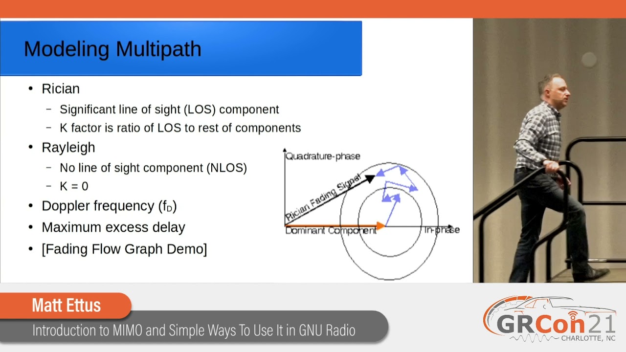




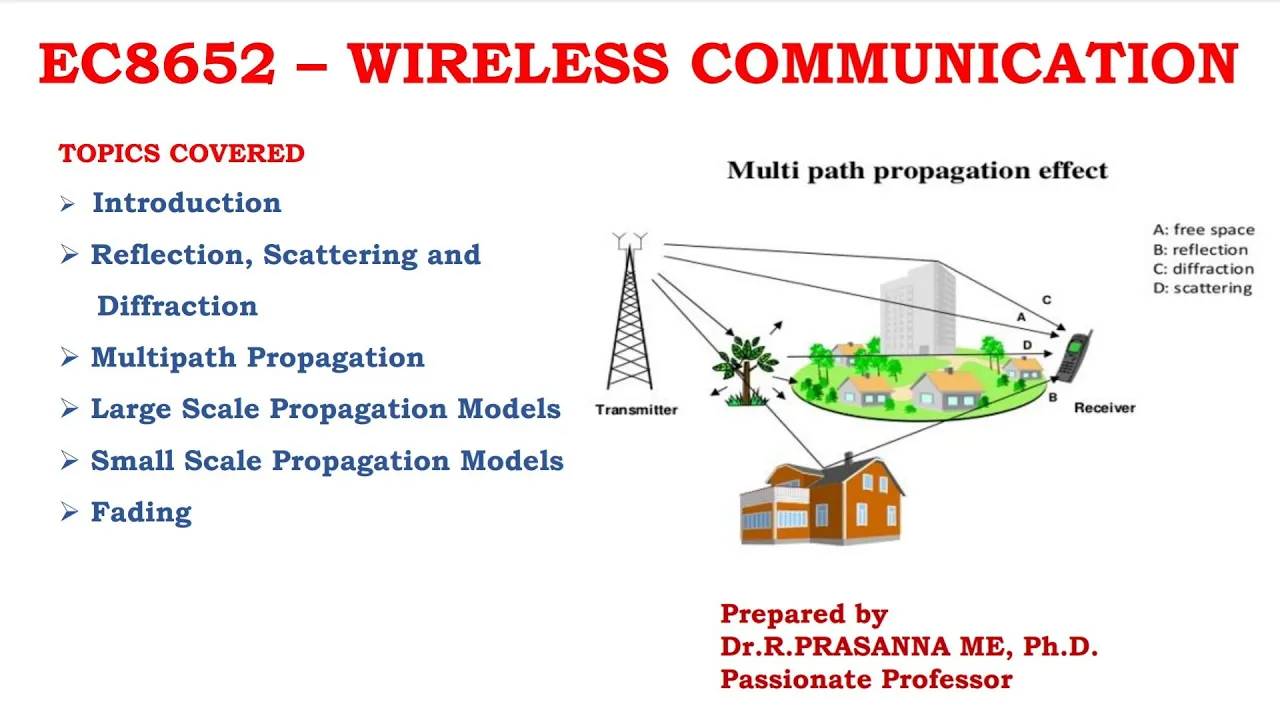
In narrowband wireless communication, small scale fading occurs when multiple propagation paths with different delays and Doppler shifts combine coherently at the receiver, causing rapid power fluctuations. The channel can be modeled as a superposition of multipath components, each characterized by its own delay, amplitude, and Doppler shift. The Doppler shift depends on the carrier frequency, receiver velocity, and angle of arrival, with higher frequencies experiencing larger Doppler shifts. The delay spread, representing the time difference between the first and last path arrivals, varies by environment (10-100 ns indoors, up to 1 μs outdoors) and determines the channel's frequency selectivity.
Wireless Channel Fading: Narrowband vs Wideband Analysis
Added:Basic principles of electromagnetic wave propagation, including reflection, diffraction, and scattering.
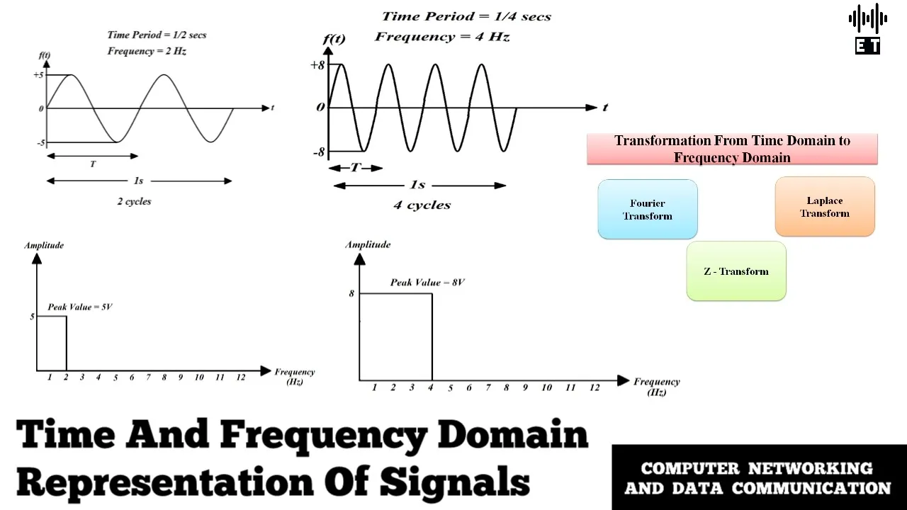
Signal representation in both time and frequency domains, including Fourier transforms and the concept of signal bandwidth.
The concept of multipath propagation and how constructive and destructive interference affect received signal strength.
Foundational probability and random processes, which are essential for understanding statistical channel modeling.
Statistical channel models such as Rayleigh, Rician, and Nakagami-m fading distributions.
Fading mitigation techniques, including diversity schemes (space, time, frequency) and MIMO (Multiple-Input Multiple-Output) systems.
Orthogonal Frequency Division Multiplexing (OFDM) and how it combats frequency-selective fading by partitioning wideband channels.
Design and implementation of channel equalization techniques and RAKE receivers to resolve multipath delay spread.
1.2K views7likes15:55Original Release: 2023-08-27
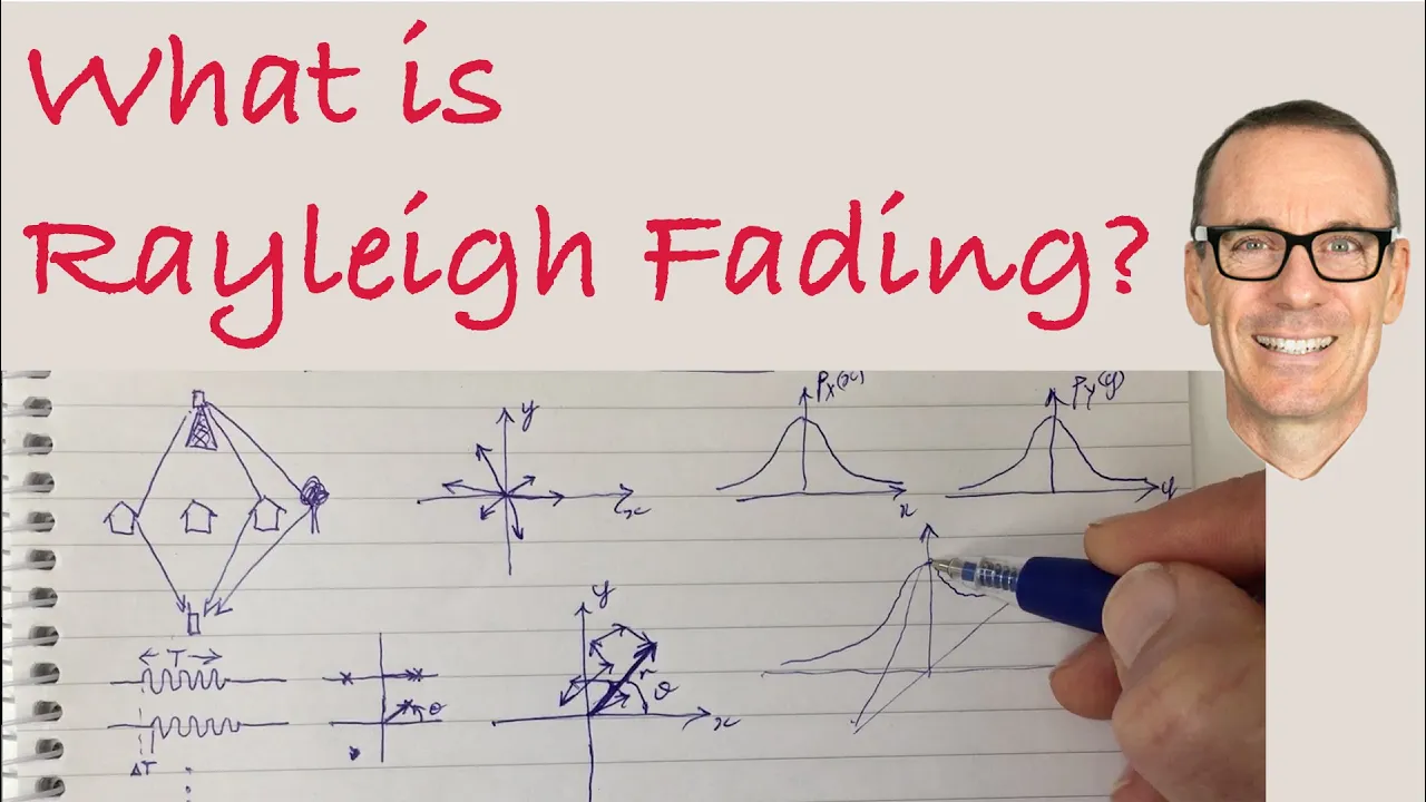
so welcome to this uh third lecture on wireless communication where we continue talking about the wireless channel the topics I will cover today are to some extent covered in chapter three of the book and I really recommend that you read these highlighted sections from the book today we will talk about wideband and narrow band communication Doppler shifts resolvable paths the general formula for time varying channels which we've briefly covered in lecture one uh and also we talk a little bit about really and risan channels we'll also cover autocorrelation power spectral D density of WID St stationary fitting processes this is what we've seen last time so the channeling principle is given by Maxwell's equations which you can simplify to rracing which you can further simplify through the combination of three effects first effect is path loss this is the deterministic decay of the power with distance uh given by this equation here where gamma is called the path loss exponent that determines the slope of this yellow curve then we have shadowing which is due to large scale variations of the power in the environment so I can show this by this curve here so large scale variation in the of the power this is modeled as a log normal random variable which in the DB domain is a normal random variable or gussian random variable um here the mean is zero because the the average power is given by the power due to path loss and this is then the additional power due to shadowing has mean zero and a certain variance Sigma squared here so then I could write the total receive power due to path loss and shadowing by this expression the DP domain the final effect um is multipath fading and these are very small scale variations of the received power on the order of a wavelength and this is due to mobility and small changes in the environment such as Reflections and scattering off of object and this will also be modeled as random and this will be the main topic of today we also saw this slide last time where we uh talk about wideband and narrow band communication so wideband means that we sent a very short pulse at the transmitter in narrow band we sent a very broad pulse at the transmitter so this will be time if you send this very short pulse you will receive um all of these multipath Reflections here so each of these paths corresponds to Something in the environment the bounce of some object when the transmit pulse is very long like shown on the right you will receive all of these pads lumped together so this total duration would be the same but it would just appear as one path if the receiver is moving a little bit or something is changing the environment in the wideband case things would look more or less the same small variations but for the narrow band case the power can fluctuate a lot because all of these paths they will add up coherently or incoherently and lead to large fluctuations so this means that when a user is moving then over time the power would vary so this is what is shown here on this figures on the bottom and these are two different time scales so it depends um on number of parameters how quickly this power changes over time and we will cover this soon now the basics for the multipad fading is a Doppler shift so as you may recall when a transmitted signal is sent at some frequency and um a receiver is moving with some velocity in some direction the received signal will arrive with a Doppler shift and this is the same effect that you have when you an ambulance Drives By when it's coming towards you the frequency is increasing when it's driving away from you the frequency is decreasing this Doppler shift depends on the carrier frequency speed of light and the angle of the transmitter with respect to the receiver so this angle is shown here and this can be greater or uh smaller than zero depending of the Velocity well depending on this angle Theta of course we see that um when the velocity increases this means that the Doppler shift will increase also when Lambda decreases this also means the Doppler shift will increase this means that systems with uh small with high carrier frequencies which have smaller lambdas they will suffer from higher Doppler frequencies now to get a feeling of how important these Doppler frequencies are you can consider this example where we have a 1 GHz carrier a user moving at 75 km per hour and the question is what is the doler so you can try to solve this yourself and then come back to the video so we recall that when the carrier is 1 GHz this implies that Lambda is 0.3 M when V is equal to 75 kilometer per hour this implies that V is approximately 20 m/ second this you can do yourself and then it follows that f d which is V over Lambda at most right it can be smaller depending on the angle um this will be approximately and now this is very rough UH 60 hertz right it's 20 m/s over 0.3 M so about 60 htz now what is important that this is that this 60 hertz is way smaller than this one gahz so it's a very small deviation here but when you increase the carrier a lot then this deviation will become more important right so if you take a 30 GHz carrier then you can compute a doler and it will be much larger now in practice you will not just have this line of sight path from transmitter to receiver but your signal will bounce of objects in the environment each of these will have a different angle so each of these will have a different doler shift this is what we will see now so now we consider a scenario okay let me try to draw a picture where there's a transmitter somewhere here there's your car somewhere here in some direction there's some angle Theta for the line of s path and then in the environment there's some objects and for each of object there's a path going to the receiver so let's say the receiver has an antenna here on the back right so each of those paths has its own angle data each of them will have its own propagation delay Tow and each path will have its own path loss and shadowing Alpha right and we have multiple paths so we'll index them with n good so now in the more mathematical terms we have here the transmitted signal which is upconverted and uh so U of T is the complex baseband signal s oft is the pass band signal this goes over the environment and then we look what the receiver observes so in line of sight which means that there's only one path from the transmitter to the receiver what the receiver will observe over time is the transmitted signal which is delayed it is delayed because the user is moving so over time this delay will increase in this case user is moving further away so that's why we have this to of T the signal is also affected by a power loss and this here is shown as path loss and shadowing so here maybe it's also important to mention that this Alpha is the amplitude this means that Alpha squar will be the power right so when we talked about pthos and shadowing last time we it was referring to power so the amplitude is the square root of that and this Pathos and shadowing will also change over time right because when you're moving further away the pthos will increase and then the shadowing is a random process this will vary and then finally you have the um frequency component so you have the received signal which has the same carrier frequency but it's subject to a Doppler shift and then of course this T will become T minus to right because the signal again is delayed and this also manifest itself in the face so let me remove this so this is what the receiv receiver will see as a received passband signal plus noise of course now you see again there's all these effect the delay the amplitude and the Doppler now each of these are not changing very quickly right the delay changes based on the speed it's kind of move changing slowly p is also changing slowly and the Doppler shift in this case could be constant so what now gives rise to this rapid variations of the channel this is really due to the fact that in practice you have many paths so let's say you have n pads so in this case we had one we had n equal to five pths then since this communication system is linear what we will receive is the superposition of all of these paths so we will receive the sum of these paths and each of these paths is of the same shape as a line of side path but with its own delay own amplitude and own Doppler shift and again we have the delay so what I do now is I pull out this uh a to the^ J 2 pi fct right I pull this out put it here so then what is remaining this here would be the complex basement so this is the received signal in complex basement ignoring the noise now what we would like is to have an expression as we've seen in the first lecture of this form right where you have the transmit signal and then you have the time varying Channel and now you can easily see that the only possible expression for this C of to and T is given here so it is the same as what is in the green box so a superposition of paths the only thing that's different is that I have these Delta functions here so the channel is basically a sequence of pulse impulses with different delay different amplitude and different phase uh maybe it's also good to mention what this pH is so let's see here f n of t will be everything in the exponent here except to the thing that I pulled out so it will be 2 pi f n d t minus to n t Min - 2 pi FC to n t and now it's important to recall that this value is very large right this is many gig Hur so this means that this will be uh rapidly fluctuating right as soon as you move a wavelength your phase will rotate 2 pi all right anyway so in the end we get this uh time varying uh well this actually the time varying Channel and to verify this if you plug this into here you will find what is in the green box so as we already hinted that before the the channel breaks down into two cases the the narrow band and the wide band regime so here we'll try to make this a bit more mathematical so in this box here this is the physical channel so this is what's given by by nature but and also based on the the velocity that you're working over um well it partially depends on the only thing that matters here actually is this fre the carrier frequency so this is what matters here because this will affect how this channel looks like and in this channel there are two Dimensions there's the there's to and T so the delay domain and the time domain and I'll show you a picture of this in the next slide so we can study this channel in two ways we can um well let's first go to the left at a certain time we can study the channel in the delay domain okay so this would look something like Tow and then we have C of to at some time T and this channel would have some impulses like this right where the first one could be the line of side path and then different Reflections for this channel we introduce a concept called the delay spread this is expressed in seconds and it's a time between the first and the last arrival now I made my figure a bit too small to make it really useful so let me move it here this is to this is C of to at sometime T so this is fixed you can see this say this is the channel today and then the channel tomorrow could be something different and this consist of some impulses like this and then this time here is called the delay spread now um this delay spread actually tells you a little bit also about the propagation environment so for instance um let's see if for a good example let's say indoors right in let's say in a lecture hall the difference between the first and the last p path could be about let's say 30 m right because there's a line of side path and then it bounces off some wall and comes back to you and the difference between those two paths is 30 m so this would correspond to um 10 nond NS so this means that in indoor environments you know that are not too complex maybe 10 100 nond is reasonable Outdoors Outdoors um you could have maybe a path that bounces off a mountain and comes back to you then it could be 3 km right and then it would be a delay spread of what would it be 100 times what I had before so 1 microc okay so the delay spr tells you a lot about the environment I think my first 15 minutes are up so let me see I can break the video and two see you soon
Up Next

8:36
Anatomy of a Wind Turbine: Key Components Explained
@windfarmguy7286
241 views•2023-01-14

30:32
Ultrasonic Transducers: Resonant Frequency Measurement and Horn Design
@imajeenyus42
229.9K views•2017-02-22

54:16
Polymer Environmental Degradation: Mechanisms & Stabilization
@iit
1.8K views•2012-07-10

33:39
How a Student's Question Saved a NYC Skyscraper from Collapse
@veritasium
22.8M views•2025-04-26
Related Study Plans & Knowledge Roadmaps
Structured learning paths in Engineering
engineering
Building Acoustic Levitators: Physics & Arduino
01The Physics of Sound and Standing Waves
02Piezoelectric Transducers and H-Bridge Drivers
03Arduino Programming: Generating 40 kHz Signals
+ 2 more learning modules
14h5 modules
Explore Roadmap
engineering
Building Peltier Cloud Chambers: Particle Tracks
01Cosmic Rays & Cloud Chamber Physics
02Thermoelectric Cooling (TEC) Fundamentals
03Custom Liquid-Cooling Loop Design
+ 2 more learning modules
18h5 modules
Explore Roadmap
engineering
Yagi-Uda Antennas: Modeling, Build & VNA Test
01Introduction to RF and Antenna Fundamentals
02Yagi-Uda Antenna Design Principles
03Antenna Modeling and Simulation in 4NEC2
+ 2 more learning modules
18h5 modules
Explore Roadmap
engineering
ECG Monitor Design: Op-Amps, Filters & Noise
01Electronics & Breadboard Basics
02Op-Amps and Instrumentation Amplifiers
03Bioelectricity and ECG Fundamentals
+ 2 more learning modules
18h5 modules
Explore Roadmap