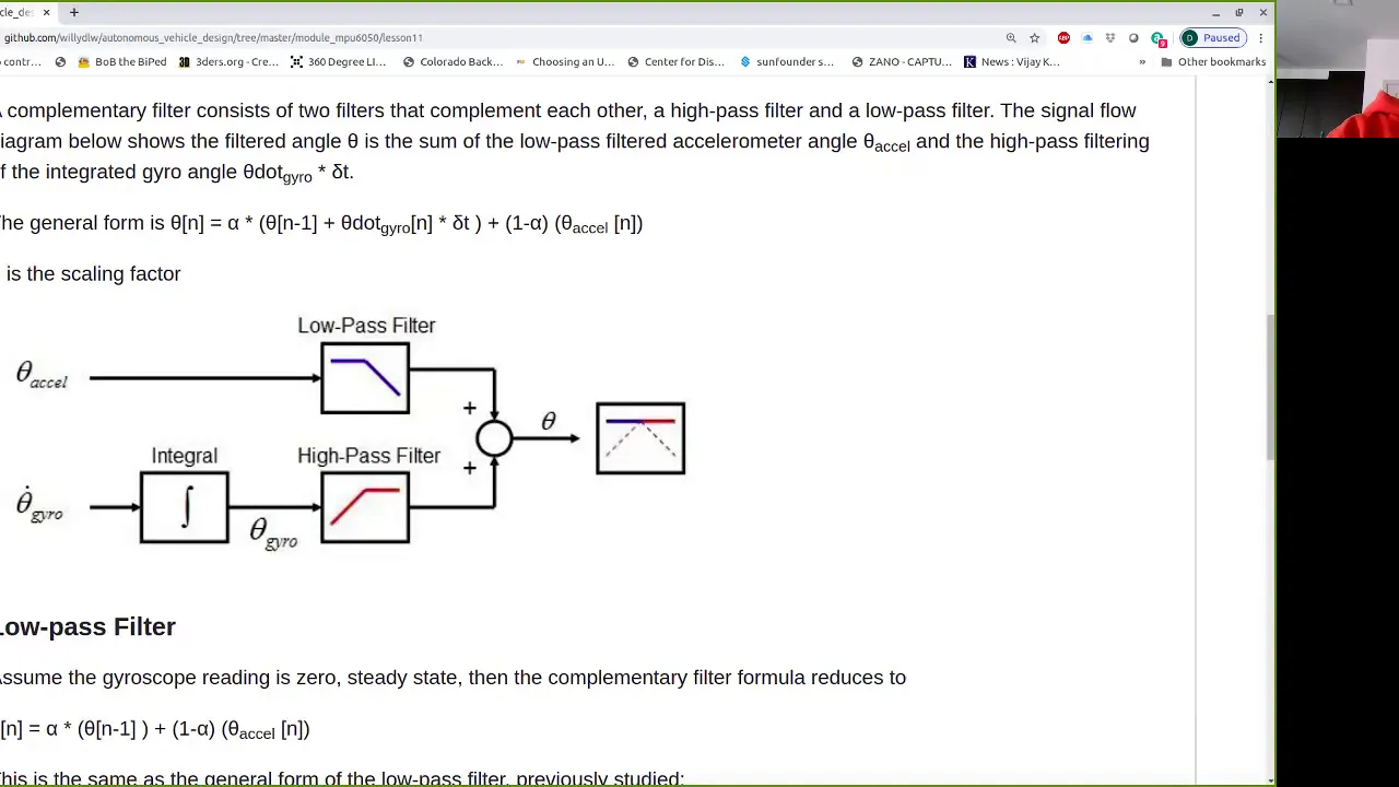
A complementary filter combines accelerometer and gyroscope data to provide more accurate and stable orientation measurements than either sensor alone; accelerometers are sensitive to disturbances but stable over time, while gyroscopes drift systematically but respond quickly to rotation, making their combination particularly effective for real-time motion tracking applications.
MPU-6050 IMU Data Fusion with Complementary Filter | Arduino & Processing
Added:Deep Dive
Basic understanding of IMU sensors, specifically the operational differences between an accelerometer (measures gravity and linear acceleration, prone to noise) and a gyroscope (measures angular velocity, prone to integration drift).

Intro to Inertial Measurement Units (IMU)
46.1K
An Inertial Measurement Unit (IMU) is a sensor system that measures orientation and motion using gyroscopes (which detect angular rotation rates but suffer from bias and drift requiring correction algorithms like Kalman filters) and accelerometers (which measure linear acceleration including gravity to determine tilt angles but require filtering to reduce noise); IMUs are classified by their sensor accuracy, with hobbyist-grade units having biases around 0.01g and 100°/hour, while high-end aerospace IMUs achieve biases below 0.00001g and 0.1°/day, and sensor fusion techniques combine multiple sensor readings to improve overall measurement accuracy.
Click to watch →
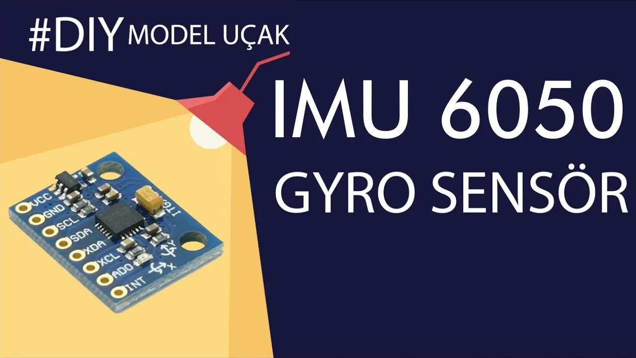
Arduino Severler: Bu Sensörü MUTLAKA Öğrenmelisiniz! | MPU6050 ve Arduino Kullanımı | JLCPCB
10.1K
The gyroscope measures angular velocity (degrees per second), indicating rotation rate. Since Earth rotates, stationary sensors detect constant angular velocity, causing drift over time. The accelerometer measures acceleration forces, detecting gravity when stationary. When tilted, gravitational force vectors shift across axes. Accelerometer readings remain stable without drift, while gyroscopes accumulate error from Earth's rotation and other factors.
Click to watch →

Arduino 9 Axis, 9 Degree of Freedom Inertial Measurement IMU
34K
This section covers the foundational principles of inertial measurement systems. A 9-DOF IMU combines 3-axis accelerometers (measuring linear acceleration), 3-axis magnetometers (measuring magnetic fields), and 3-axis gyroscopes (measuring angular velocity). Raw accelerometer signals show clear acceleration spikes along X, Y, and Z axes, but attempting to calculate position by double-integrating acceleration fails catastrophically due to accumulated noise. Accelerometers can measure tilt angles using arcsine on calibrated signals, but they become unreliable during dynamic motion because any additional acceleration creates erroneous readings beyond the static gravity vector. Gyroscopes provide clean angular velocity signals with minimal noise, making them excellent for detecting rotational changes, but integrating these signals to obtain angular position causes significant drift over time—even when stationary, hundreds of degrees of drift can accumulate within minutes.
Click to watch →

How robots navigate the world: Sensors, Mapping & Localization – A Talk by Naveen Arulselvan
1.1K
Inertial Measurement Units (IMUs) contain accelerometers and gyroscopes that measure linear acceleration and angular velocity respectively. Accelerometers detect forces acting on a suspended mass, allowing calculation of linear acceleration by resolving forces perpendicular to gravity. Gyroscopes measure rotational rates. Both sensors have significant noise: accelerometers produce high-frequency noise, while gyroscopes drift slowly over time. These complementary characteristics lead to complementary filter techniques that combine both sensor types for improved orientation estimation.
Click to watch →

How a Quadcopter Works - Flight Mechanics, Components, & Sensors (2)
95.5K
The IMU (Inertial Measurement Unit) contains two sensors: the accelerometer measures linear force exerted on the quad (linear acceleration), and the gyroscope measures rotational motion. Together, they measure linear and rotational forces but do not know the absolute position or orientation (whether the quad is upright or upside down).
Click to watch →
Deep Dive
Fundamentals of Arduino programming, including reading sensor registers over I2C communication and working with basic data structures.

I2C Communication Protocol and Arduino Implementation Tutorial
1.6M
Implementing I2C communication with Arduino requires understanding device addresses and register mappings. Each sensor has a unique I2C address found in datasheets or via the I2C Scanner sketch. Internal register addresses specify where data is stored—for example, the ADXL345 accelerometer stores X-axis data across registers 0x32 and 0x33. The Arduino Wire library provides essential functions: Wire.begin() initializes communication, Wire.beginTransmission() specifies the target device, Wire.write() sends register addresses, Wire.endTransmission() completes sending, Wire.requestFrom() requests data, Wire.available() checks byte availability, and Wire.read() retrieves data bytes. Raw sensor data requires mathematical conversion to obtain meaningful physical measurements, demonstrating how hardware communication protocols enable complex sensor integration through standardized two-wire interfaces.
Click to watch →

Tutorial 07 for Arduino: I2C Communication and Processing
461.9K
Programming I2C communication on Arduino requires importing the Wire library and initializing with Wire.begin(). The process involves: (1) beginTransmission() with the target device address, (2) sending the register address using send(), (3) ending transmission with endTransmission(), (4) requesting data with requestFrom() specifying the number of bytes, and (5) reading the response with receive(). For temperature conversion from Celsius to Fahrenheit, use F = C × 9.0/5.0 + 32.0 with floating-point arithmetic to maintain precision. Serial.print() outputs values to the computer terminal, allowing real-time monitoring of sensor readings.
Click to watch →
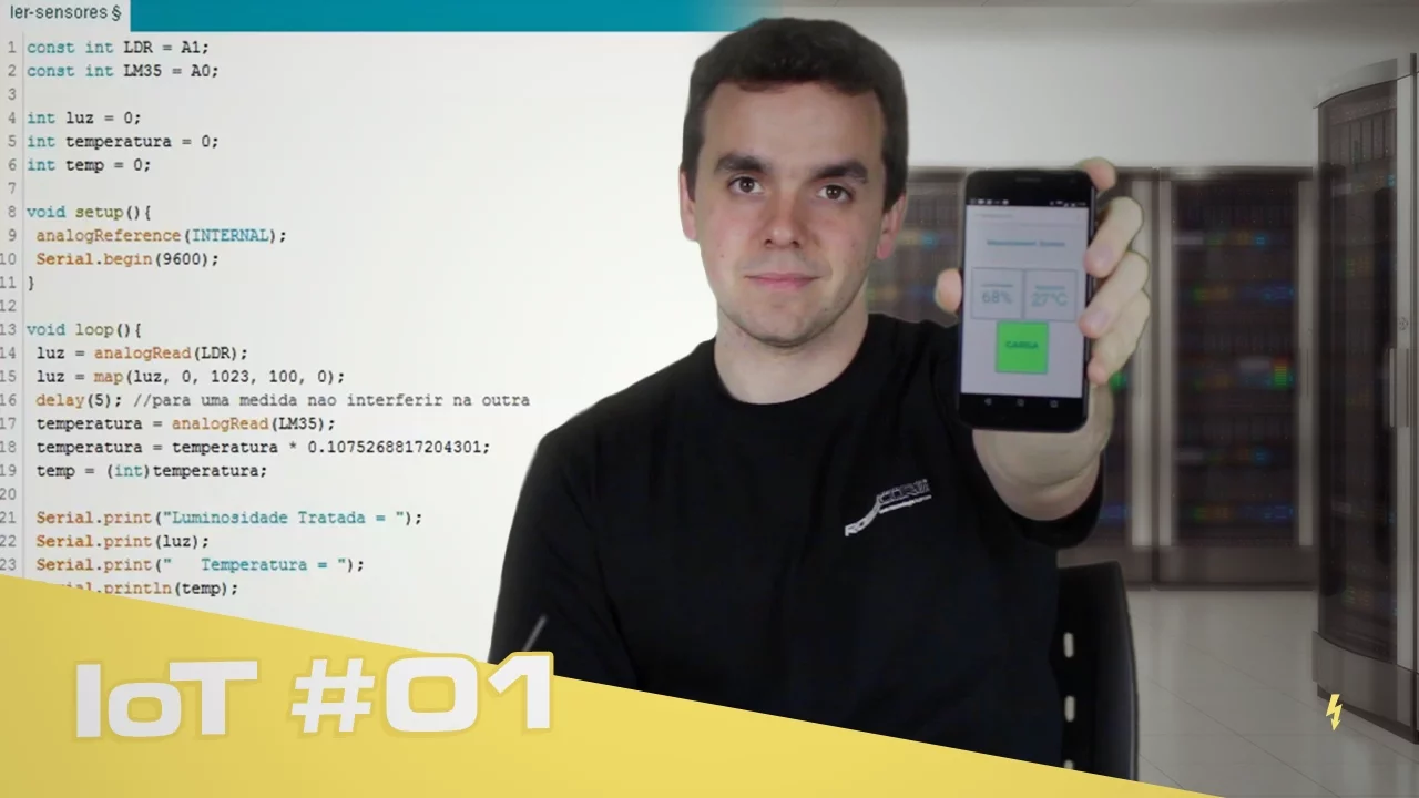
Projeto Internet of Things // Parte 01
42.4K
This segment covers the foundational Arduino code structure for reading sensors. The setup() function initializes pins and serial communication, while loop() handles continuous sensor reading. Constants are declared for fixed pin numbers (LM35 on A0, LDR on A1), and variables store sensor readings. The critical concept of analog reference voltage is explained: the default 5V reference wastes the voltage range for sensors like LM35 (max 1.12V). Using internal reference (1.1V) provides better precision. For Arduino Uno/Blackboard, use 'internal'; for Arduino Mega, use 'internal1v1'.
Click to watch →
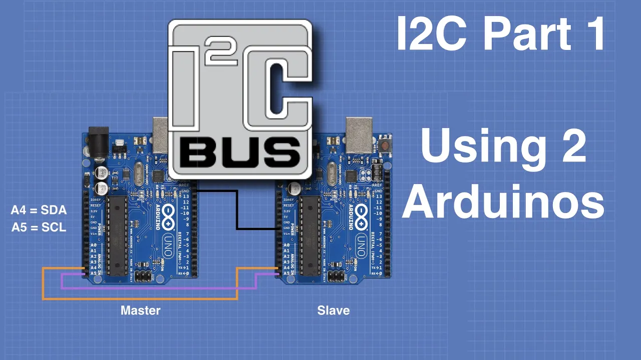
I2C Part 1 - Using 2 Arduinos
465.6K
I2C (Inter-Integrated Circuit) is a serial protocol for low-speed two-wire communication, originally developed by Philips in 1982 for television manufacturing. It uses three physical connections: VDD (power, 3.3V/5V), SDA (bi-directional data), and SCL (clock signal) with pull-up resistors. The bus supports multiple speed modes: standard mode (100kHz), fast mode (400kHz), high-speed mode (3.4MHz), and ultra-fast mode (5MHz). Devices use a 7-bit addressing scheme supporting up to 128 slaves, with variants including TWI and SMBus. On Arduino, SDA is A4 and SCL is A5 on Uno, with pull-up resistors needed externally. The Wire library handles I2C operations, with master mode using Wire.begin() and slave mode using Wire.begin(slaveAddress). Master sends data via beginTransmission(), write(), endTransmission(). Slave receives data through onReceive() event function. Master requests data via requestFrom().
Click to watch →

28 july iot Practical Paper Solution | O Level IoT Practical Exam Analysis | IOT M4R5 PRACTICAL PR4
6.7K
Arduino programming requires setup() and loop() functions. Setup runs once, loop runs repeatedly. Analog sensors use analogRead() (pins A0-A5, values 0-1023), digital sensors use digitalRead() (pins 0-13, values HIGH/LOW). Serial Monitor displays readings using Serial.begin(9600). Digital pins require pinMode() configuration (INPUT for sensors, OUTPUT for actuators). Delay() controls timing in milliseconds.
Click to watch →
Deep Dive
Basic trigonometry and coordinate geometry concepts, particularly understanding Euler angles (pitch, roll, and yaw) and using trigonometric functions like arctangent to calculate tilt.
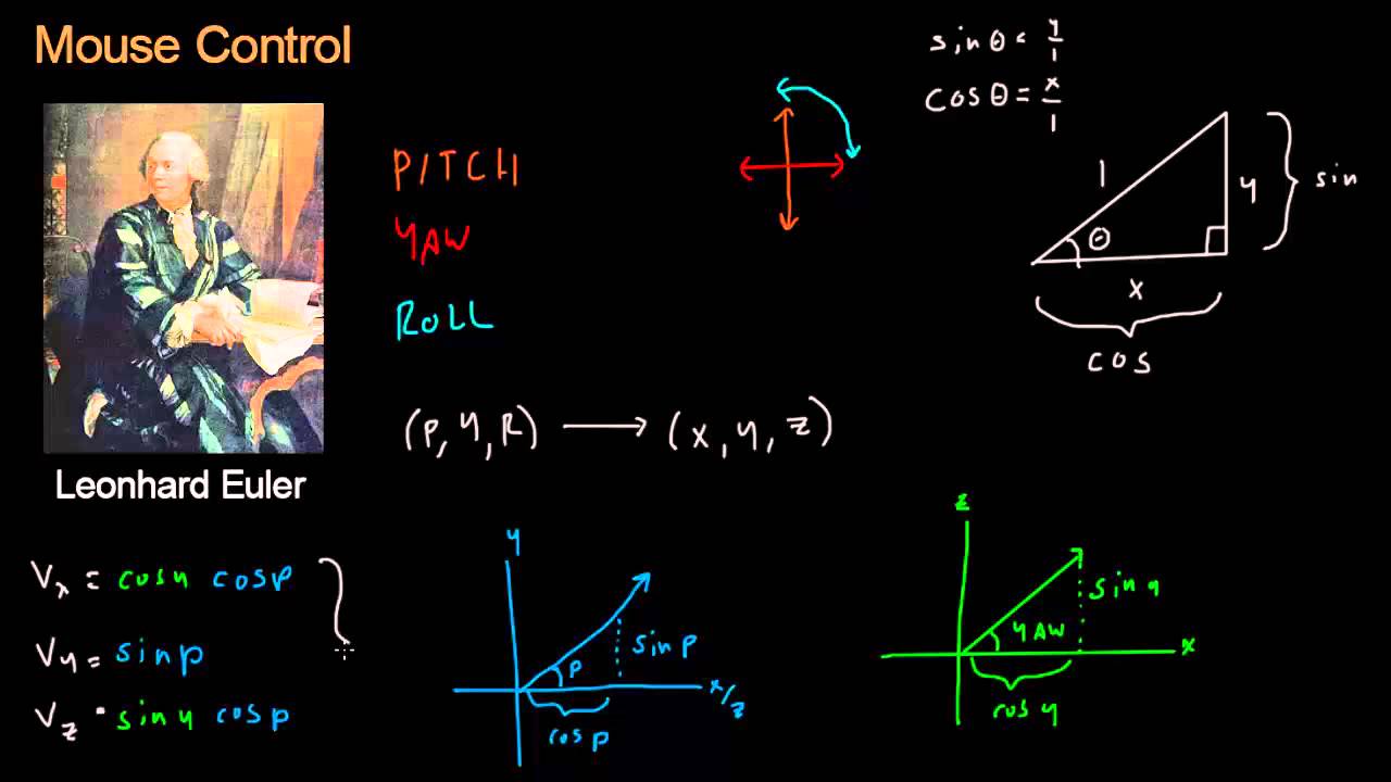
Math for Game Developers - Mouse Control (Euler Angles)
69.5K
Euler angles (pitch, yaw, and roll) can be converted to a 3D view vector using trigonometric functions: the X component equals cos(yaw) × cos(pitch), the Y component equals sin(pitch), and the Z component equals sin(yaw) × cos(pitch), where pitch controls up/down mouse movement, yaw controls left/right mouse movement, and roll handles side-tilting; this conversion requires scaling by cos(pitch) to ensure the vector correctly represents the viewing direction when looking straight up.
Click to watch →

9-Axis IMU LESSON 6: Determine Tilt From 3-axis Accelerometer
36.2K
SOHCAHTOA (Sine=Opposite/Hypotenuse, Cosine=Adjacent/Hypotenuse, Tangent=Opposite/Adjacent) provides the mathematical framework for tilt measurement. For pitch angle, the formula is theta = arctan(a_x/a_z), where a_x is X-axis acceleration and a_z is Z-axis acceleration. This relationship holds because the tangent of the tilt angle equals the ratio of the X-component to the Z-component of the gravitational vector. The approximation works best between 0-45 degrees.
Click to watch →
Euler Angles and the Euler Rotation Sequence
59.6K
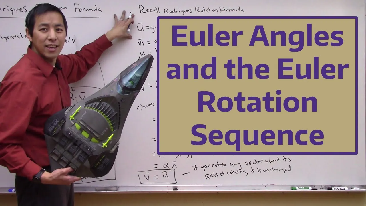
Euler angles are three angles developed by Leonard Euler for describing object orientation in space. Using an aircraft example, we define two coordinate frames: the reference frame (Northeast Down - NED) and the body frame attached to the aircraft's center of gravity. The Euler rotation sequence involves three consecutive right-handed rotations: (1) yaw about the z-axis to get frame F1, (2) pitch about the common y-axis to get frame F2, and (3) bank about the common x-axis to reach the body frame. Each rotation step is represented by a 3x3 rotation matrix: R_z(ψ) for yaw, R_y(θ) for pitch, and R_x(φ) for bank. The complete transformation from reference to body frame is C_BV = R_x(φ) × R_y(θ) × R_z(ψ), yielding the Direction Cosine Matrix (DCM). Aerospace conventions specify that Euler angles are ordered as φ (bank), θ (pitch), ψ (yaw), even though the actual rotation sequence is yaw-pitch-roll (ZYX).
Click to watch →
Flight Dynamics (9/9): 3D transformation w/ Euler Angles
426
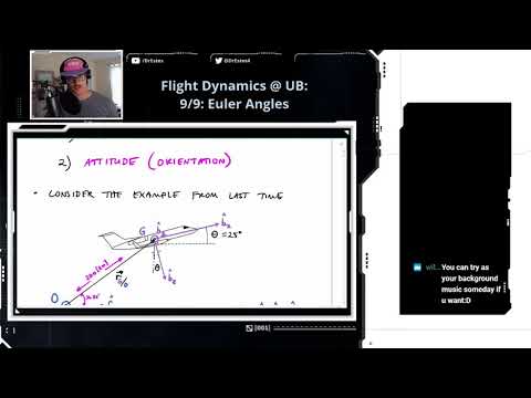
Given a rotation matrix, Euler angles can be recovered using specific formulas: (1) c = arctan2(R[1,2], R[1,1]) - this gives the yaw angle from the first row elements; (2) θ = -arcsin(R[1,3]) - this gives the pitch angle from the third element of the first row; (3) φ = arctan2(R[2,3], R[3,3]) - this gives the roll angle from the third column elements. These formulas allow conversion between the matrix representation and the angle representation of orientation.
Click to watch →

Curso 2015-16. Ángulos de balanceo, cabeceo y giñada (2)
2K
This video explains how to calculate the three Euler angles (roll/chi, pitch/tita, and yaw/phi) from a rotation matrix representing the roll-pitch-yaw sequence (rotation around X-axis by chi, then Y-axis by tita, then Z-axis by phi). The method involves two cases: when cos(tita) is positive (quadrants 1 and 4), the angles are calculated as chi = arctan(r32/r33), tita = arctan(-r31/√(r11²+r21²)), and phi = arctan(r21/r11); when cos(tita) is negative (quadrants 2 and 3), the calculations use negative values for the denominator. The key insight is that r11² + r21² = cos²(tita), allowing determination of the pitch angle's quadrant, which then affects how the other angles are computed.
Click to watch →
Deep Dive
Elementary familiarity with the Processing development environment and Serial communication protocols to stream data between hardware and software.

Design Arduino GUI with Processing 4 - Beginner's Guide | PART-1
7.4K
The serial library enables communication between Processing and Arduino. Import processing.serial.*, use serial.list() to find available ports, then create Serial instances with new Serial(parent, portName, baudRate). Send data using write(), place write() inside draw() for continuous transmission, and add \n for message separation. On Arduino, use Serial.begin(baudRate), pinMode(), and evaluate Serial.read() in loop() to control hardware based on received data.
Click to watch →
Arduino invia dati a un'applicazione Processing - #70
15.5K
This section covers the complete process of establishing serial communication between Arduino and Processing. Arduino sends data through its serial port using stamper() in the loop function. Processing receives this data by importing the Serial library (import processing.serial.*), creating a Serial object, and using serial.readStringUntil('\n') to read incoming data. The baud rate must match between both devices (typically 9600). This communication channel enables interactive applications where Arduino controls Processing graphics and vice versa.
Click to watch →
Tutorial 07 for Arduino: I2C Communication and Processing
461.9K
Processing is a visual programming language for creating interactive graphics and animations. To prepare for serial communication: (1) Create custom fonts via Tools > Create Font, selecting a font style and size (e.g., Agency FB at 200), which generates .vlw files; (2) Load fonts using PFont font = loadFont("fontname.vlw"); (3) Set up the canvas with size(width, height); (4) Initialize serial communication using SerialPort port = new SerialPort(this, "COM3", 9600); (5) Configure buffering with port.bufferUntil('.') to wait for complete data packets terminated by a period. The draw() function continuously refreshes the display, making it ideal for real-time data visualization.
Click to watch →

Comunicacion serial con processing 01
5K
This section demonstrates the complete data flow between Arduino and Processing. Arduino sends data using Serial.print() and Serial.println() with matching baud rates. Processing reads incoming data using miPuerto.read() and displays it in the console. The demonstration shows sending integer values (0, 1, 70, 255) and explains that serial communication is limited to 8-bit values (0-255), as values exceeding 255 will be read incorrectly.
Click to watch →

Tutorial 06 for Arduino: Serial Communication and Processing
858.8K
Processing is a flexible programming environment and language designed for visual arts and graphics programming. It shares its syntax with Java and is widely used for creating interactive visual projects. The Arduino programming environment was heavily influenced by Processing, making it familiar to Arduino users. Processing can be downloaded from processing.org and run directly from the extracted folder without installation. It provides a simple interface for creating graphical applications that can interface with hardware through serial communication.
Click to watch →
Prerequisite Knowledge
- Concept 01Basic understanding of IMU sensors, specifically the operational differences between an accelerometer (measures gravity and linear acceleration, prone to noise) and a gyroscope (measures angular velocity, prone to integration drift).
- Concept 02Fundamentals of Arduino programming, including reading sensor registers over I2C communication and working with basic data structures.
- Concept 03Basic trigonometry and coordinate geometry concepts, particularly understanding Euler angles (pitch, roll, and yaw) and using trigonometric functions like arctangent to calculate tilt.
- Concept 04Elementary familiarity with the Processing development environment and Serial communication protocols to stream data between hardware and software.
Subsequent Learning
- Step 01Implementation of advanced state estimation and data fusion algorithms, such as the Kalman Filter or Extended Kalman Filter (EKF), for superior noise rejection.
- Step 02Transitioning from Euler angles to Quaternions for 3D orientation representation to prevent mathematical singularities like gimbal lock.
- Step 03Integrating a magnetometer (upgrading to a 9-DoF system) to calculate an absolute heading/yaw and implementing Madgwick or Mahony filters.
- Step 04Applying filtered orientation data to closed-loop control systems, such as PID-controlled self-balancing robots, active camera gimbals, or drone flight controllers.
Sensor Fusion
Sensor Fusion
0:07Playing Section
- 1
Demonstrates MPU 6050 IMU with accelerometer and gyroscope wired to Arduino.
- 2
Shows raw sensor outputs: jittery accelerometer and drifting gyroscope data.
- 3
Highlights complementary filter for smooth, accurate orientation tracking.
Kalman Filtering and Advanced State Estimation Algorithms
While complementary filters are popular in beginner Arduino projects due to their simplicity and low computational overhead, they suffer from significant limitations in dynamic environments. A complementary filter relies on a fixed, hand-tuned weight (gain) to merge gyroscope and accelerometer data. This rigid approach struggles to handle vibration, translational acceleration, and rapid, erratic movements, which introduce orientation errors. To overcome these limitations, advanced applications utilize Kalman Filters (specifically Extended Kalman Filters) or Madgwick/Mahony algorithms. The Kalman Filter dynamically estimates the optimal state by modeling system and sensor noise in real-time, providing vastly superior accuracy in highly dynamic conditions at the expense of computational complexity. Alternatively, the Madgwick filter uses a gradient descent algorithm that delivers Kalman-like accuracy with computational efficiency near that of a complementary filter, making it a highly effective alternative for resource-constrained microcontrollers tracking complex motions.
Deep Dive
Implementation of advanced state estimation and data fusion algorithms, such as the Kalman Filter or Extended Kalman Filter (EKF), for superior noise rejection.

Kalman Filter & EKF (Cyrill Stachniss)
99.8K
The Extended Kalman Filter replaces constant matrices with Jacobians G_t and H_t of nonlinear motion and observation functions evaluated at the predicted mean. The prediction step uses the nonlinear function to predict the mean, while linearized Jacobians handle covariance propagation and Kalman gain computation. The Kalman gain exhibits intuitive behavior: perfect sensors (zero noise) yield K_t = H_t^(-1), completely overriding predictions with observations; useless sensors (infinite noise) yield K_t = 0, ignoring observations entirely. Linearization error depends on function deviation from linearity and input uncertainty magnitude. Smaller uncertainties concentrate probability mass near the linearization point, reducing approximation error.
Click to watch →

Fuse, Reset, or Reject? Handling Various Data-sources in EKF2 - Marco Hauswirth, Auterion AG
514
State estimation is fundamental to drone autonomy, feeding critical data to all control modules—failure results in crashes. The Kalman filter, invented by Rudolf E. Kalman despite initial academic rejection, provides the mathematical foundation. It operates through prediction (using propagation models with process noise) and update (incorporating measurements via innovation calculations). EKF2 extends this to drones with heterogeneous sensors: IMU for prediction, GNSS for absolute positioning, cameras for map matching, and optical flow for relative motion. The same code supports different vehicle types (quadcopters, planes, rovers). Outlier detection uses innovation statistics—test ratios determine whether measurements are fused or rejected based on threshold comparisons. This architecture enables robust state estimation despite sensor limitations and environmental challenges.
Click to watch →

I Finally Refined my Self Balancing Robot!
69.2K
The Kalman filter combines gyroscope and accelerometer readings to produce accurate tilt angle measurements by weighing sensor certainty. Gyroscopes provide smooth but drifting estimates, while accelerometers give accurate but noisy readings. The filter mathematically fuses these inputs, producing a smooth, reliable estimate suitable for real-time robot control applications.
Click to watch →

SLAM-Course - 04 - Extended Kalman Filter (2013/14; Cyrill Stachniss)
133.7K
This section details the complete EKF implementation and its practical trade-offs. The EKF replaces the original nonlinear motion and observation functions with their linearized counterparts using Jacobians evaluated at the current mean. The linearized motion model becomes x̄_t ≈ G(x̄_{t-1}, u_t) + J_G(x̄_{t-1}, u_t) × (x - x̄_{t-1}), and the linearized observation model becomes z̃_t ≈ H(x̄_t) + J_H(x̄_t) × (x - x̄_t). The EKF then applies the standard Kalman filter prediction and correction steps using these linearized models. Important considerations include: Jacobians must be recomputed at every time step as the linearization point changes; approximation quality depends on nonlinearity strength and uncertainty levels; larger uncertainties relative to the linearization region produce worse approximations; and the EKF works best for systems with moderate nonlinearities and moderate uncertainties.
Click to watch →

Kalman Filter Tutorial
135.7K
A Kalman filter is a recursive algorithm that estimates the true state of a system by combining noisy sensor measurements with predictions from a mathematical model of the system's dynamics, using a weighted average where the weights (Kalman gains) are computed based on the relative uncertainties of the predictions and measurements, allowing the filter to dynamically adjust its trust in each sensor as conditions change over time.
Click to watch →
Deep Dive
Transitioning from Euler angles to Quaternions for 3D orientation representation to prevent mathematical singularities like gimbal lock.
How to Use Quaternions
66.4K
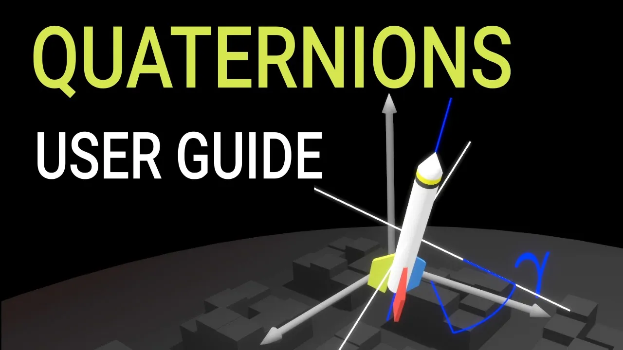
To convert Euler angles (using any scheme like zyz) to quaternions: start with the identity quaternion (which equals its own conjugate since no rotation is its own inverse). For each rotation step, multiply by the corresponding rotation quaternion. For the zyz scheme with angles Alpha, Beta, Gamma: multiply by Q_Alpha (global z-axis), then by Q_Beta (local y-axis) on the right, then by Q_Gamma (local z-axis) on the right. This method works for any Euler angle scheme without needing to look up specific conversion formulas.
Click to watch →

Rupert's Snub Cube and other Math Holes
119.8K
Euler angles represent 3D rotations as three sequential rotations around X, Y, and Z axes (yaw, pitch, roll). However, they suffer from gimbal lock (loss of a degree of freedom at certain orientations) and produce biased distributions when sampling randomly. Quaternions, which use four real numbers (w, x, y, z) representing coefficients of i, j, k imaginary units, provide a smoother representation without singularities. They correspond to points on a 4D hypersphere and avoid the problems of Euler angles.
Click to watch →
BPS.space Update - National Rocketry Conference 2019
160.2K
Flight computers use quaternions instead of Euler angles (axis-angle representation) to represent orientation because quaternions avoid gimbal lock, a phenomenon where certain orientations cannot be represented or cause loss of resolution in one axis. Gimbal lock was a problem faced by Apollo astronauts during spacecraft maneuvers. Quaternions provide computationally efficient and mathematically safe representation of three-dimensional rotations, making them ideal for aerospace applications involving complex maneuvers like those performed by reusable rockets such as Falcon 9.
Click to watch →

Math in Game Development Summit: A Visual Guide to Quaternions and Dual Quaternions
62.5K
To convert Euler angles (rotations around X, Y, and Z axes in a chosen order) to quaternions: (1) Convert each Euler angle to a separate quaternion using the axis-angle to quaternion formula; (2) Multiply these quaternions together in the correct order. This produces a single quaternion representing the combined rotation. There is no data loss in this conversion.
Click to watch →

#gimbal #6DoF #quaternion Unreal Engine 4 Tutorial: 6DoF Fixing Gimbal Lock
18.1K
Gimbal lock is a 3D rotation problem where objects lose degrees of freedom at certain orientations, preventing full 360-degree rotation. In Unreal Engine 4, this can be fixed by implementing quaternion-based rotation instead of Euler angles. The solution involves creating a Blueprint Function Library with C++ code that converts Euler angles (pitch, yaw, roll) to quaternions using functions like 'Euler to Quaternion', then applying these quaternions to the player character's rotation using 'Add Actor Local Rotation Quaternion'. This approach eliminates the singularity issue that causes gimbal lock, allowing smooth rotation in all directions.
Click to watch →
Deep Dive
Integrating a magnetometer (upgrading to a 9-DoF system) to calculate an absolute heading/yaw and implementing Madgwick or Mahony filters.
6DOF & 9DOF Sensor Fusion with Madgwick's Filter, MPU6050, HMC5883L (GY-86 Module)
28.6K
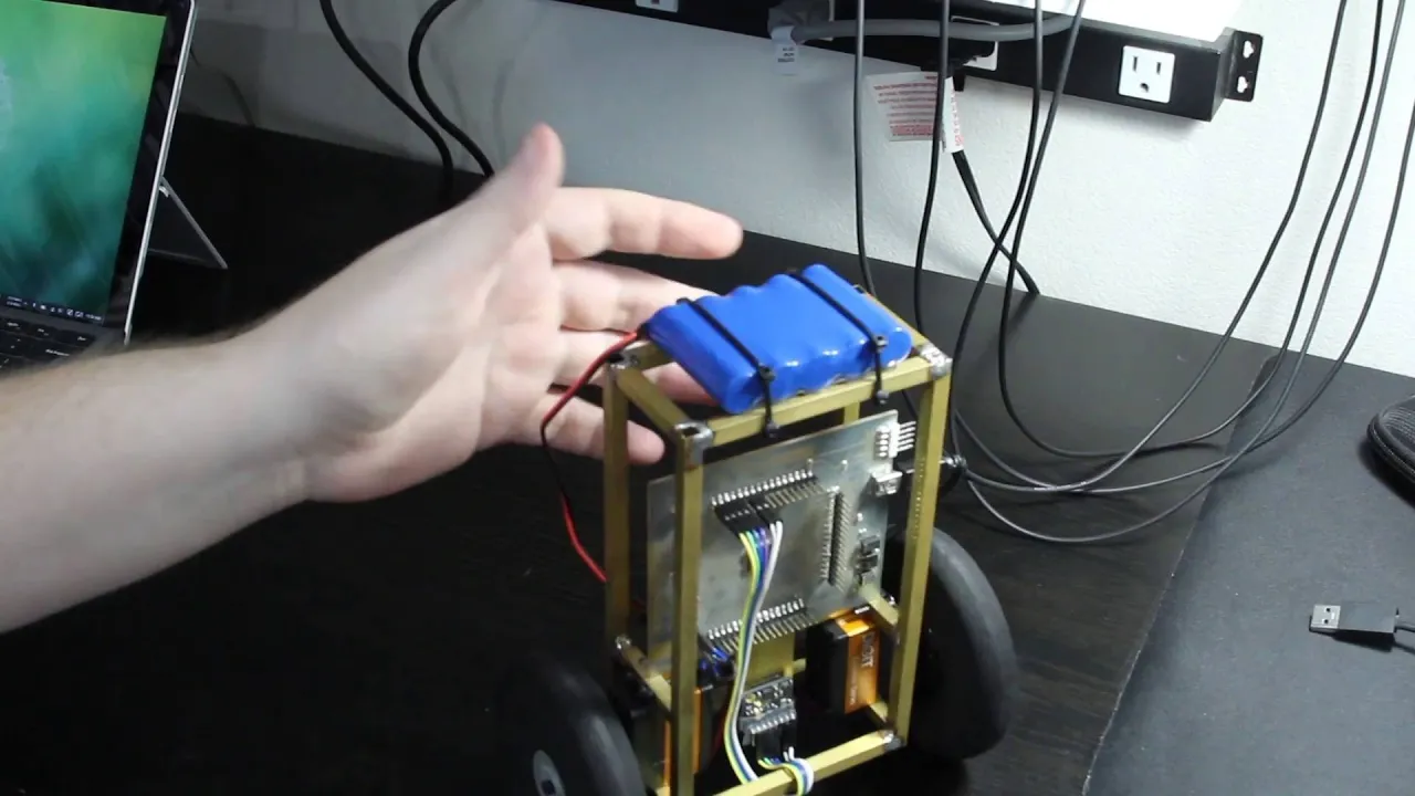
The Madgwick filter is a complementary filter algorithm for fusing IMU sensor data to estimate device orientation. It combines gyroscope and accelerometer readings (IMU mode) or adds magnetometer for 9DOF fusion. The algorithm requires two critical configurations: sample frequency (must be accurate for integration) and beta gain (controls filter responsiveness). For balancing robots, IMU mode is often preferred over 9DOF because metal chassis components distort magnetometer readings without complex compensation algorithms. The filter outputs a quaternion representing orientation, from which pitch angle can be calculated using trigonometric functions. This enables accurate attitude estimation for stabilization and control applications.
Click to watch →

How to Implement an Inertial Measurement Unit (IMU) Using an Accelerometer, Gyro, and Magnetometer
161.9K
An Inertial Measurement Unit (IMU) combines accelerometer, gyroscope, and magnetometer data through sensor fusion algorithms to determine device orientation (pitch, yaw, roll) and provide absolute acceleration values in North-East-Down coordinates; the implementation requires calibrating the magnetometer by taking median values during rotation, using an AHRS algorithm like the Mahony Quaternion Update to fuse sensor data into quaternions, converting quaternions to rotation matrices, transforming acceleration vectors to absolute coordinates, and applying magnetic declination correction for accurate heading.
Click to watch →

09 - Беспилотник на ESP32 - Основной полетный цикл
902
This section explains the sensor data processing pipeline. After validation, IMU data is converted from abstract digital values to physical quantities: accelerometer readings are converted to G-forces, and gyroscope readings are converted to radians per second. These values are then fed into the Madgwick filter, which computes quaternion orientation. Due to the 1ms cycle constraint, the filter runs every 5 IMU data cycles (every 5ms). When using a magnetometer, the filter runs once per 5ms; without magnetometer, it runs four times with the same input data. The filter receives averaged data from the previous five cycles as input. After the filter completes, the quaternion is converted to Euler angles for PID control, and the quaternion is used to transform acceleration vectors from local to global coordinates.
Click to watch →

JP’s Product Pick of the Week 12/12/23 BNO055 9-DOF Absolute Orientation IMU Breakout
2.1K
The BNO055 is a 9-DOF IMU breakout board that integrates a magnetometer, gyroscope, and accelerometer with an onboard Cortex-M0 microcontroller to perform sensor fusion calculations, automatically outputting calibrated orientation data (Euler angles and quaternions) without requiring complex calculations on the host microcontroller, making it ideal for projects requiring absolute orientation detection in 3D space.
Click to watch →

Measuring Angles and Movement with an IMU | Beginner's Guide
10.7K
A 6-DOF IMU combines an accelerometer (3 DOF translation) with a gyroscope (3 DOF rotation), providing more reliable orientation tracking than a 3-DOF accelerometer alone. Sensor Fusion combines raw readings from these two sensors to output pitch, roll, and heading. However, without a magnetometer, heading cannot be calculated accurately. A 9-DOF IMU adds a magnetometer (which measures magnetic field strength along three axes) to create a complete system. The magnetometer acts as a digital compass using Earth's magnetic field for directional tracking. Full Sensor Fusion using all three sensors provides all three axes of orientation. Not all 9-DOF IMUs perform on-board fusion - some require software implementation. The choice depends on project needs: 9-DOF offers maximum accuracy but highest cost, while 6-DOF provides good value for two-axis applications.
Click to watch →
Deep Dive
Applying filtered orientation data to closed-loop control systems, such as PID-controlled self-balancing robots, active camera gimbals, or drone flight controllers.
6DOF & 9DOF Sensor Fusion with Madgwick's Filter, MPU6050, HMC5883L (GY-86 Module)
28.6K
Madgwick's Filter is a complementary filter algorithm that fuses data from a 6DOF (gyroscope and accelerometer) or 9DOF (adding magnetometer) sensor module to provide accurate orientation estimation for balancing robots; the filter requires only two configuration parameters—the sample frequency and the gain (beta)—and outputs a quaternion that can be converted to Euler angles like pitch to determine if the robot is tipping over, enabling basic balancing control through simple proportional motor speed adjustments based on the pitch angle.
Click to watch →
I Finally Refined my Self Balancing Robot!
69.2K
The Kalman filter combines gyroscope and accelerometer readings to produce accurate tilt angle measurements by weighing sensor certainty. Gyroscopes provide smooth but drifting estimates, while accelerometers give accurate but noisy readings. The filter mathematically fuses these inputs, producing a smooth, reliable estimate suitable for real-time robot control applications.
Click to watch →

How It Balances on ONE Omni-Wheel
360.3K
Balancing robots use PID (Proportional-Integral-Derivative) controllers that run on data from inertial measurement units (IMUs) measuring pitch and roll angles. The controller differentially drives the two motors based on these measurements to maintain balance. Tuning PID parameters is critical—insufficient gain causes the robot to tip over, while excessive gain causes oscillation and instability.
Click to watch →
Build a Self-Balancing Robot: Remote & PID Control (Part 3)
34.3K
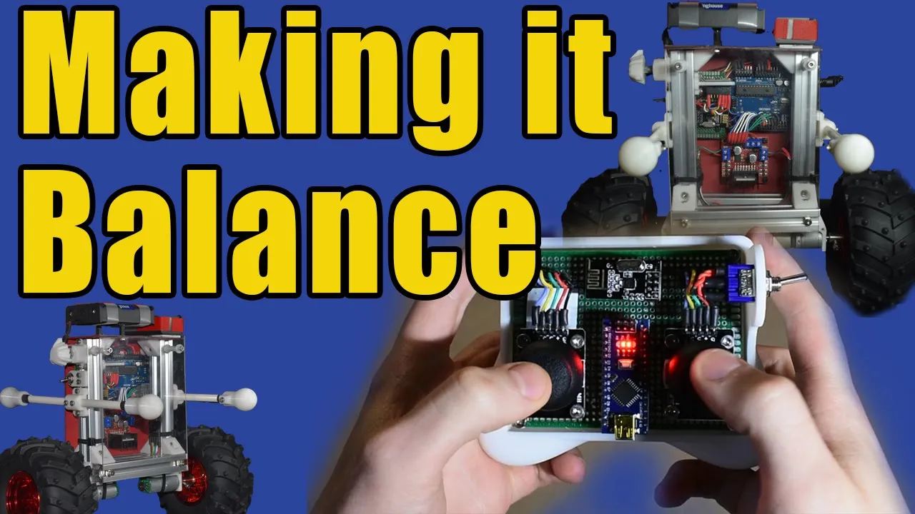
A self-balancing robot functions as an inverted pendulum that uses PID (Proportional-Integral-Derivative) control to maintain equilibrium: the proportional component responds to the current angle error, the integral component accumulates past errors to eliminate steady-state drift, and the derivative component predicts future behavior based on rate of change; the control loop continuously adjusts motor speed based on the robot's pitch angle, with the setpoint determined by both onboard sensors and remote input, while the NRF24L01 module enables wireless communication between the remote controller and the robot's Arduino-based control system.
Click to watch →
Meu primeiro projeto de robótica, um robô que se equilibra sozinho
13.3K
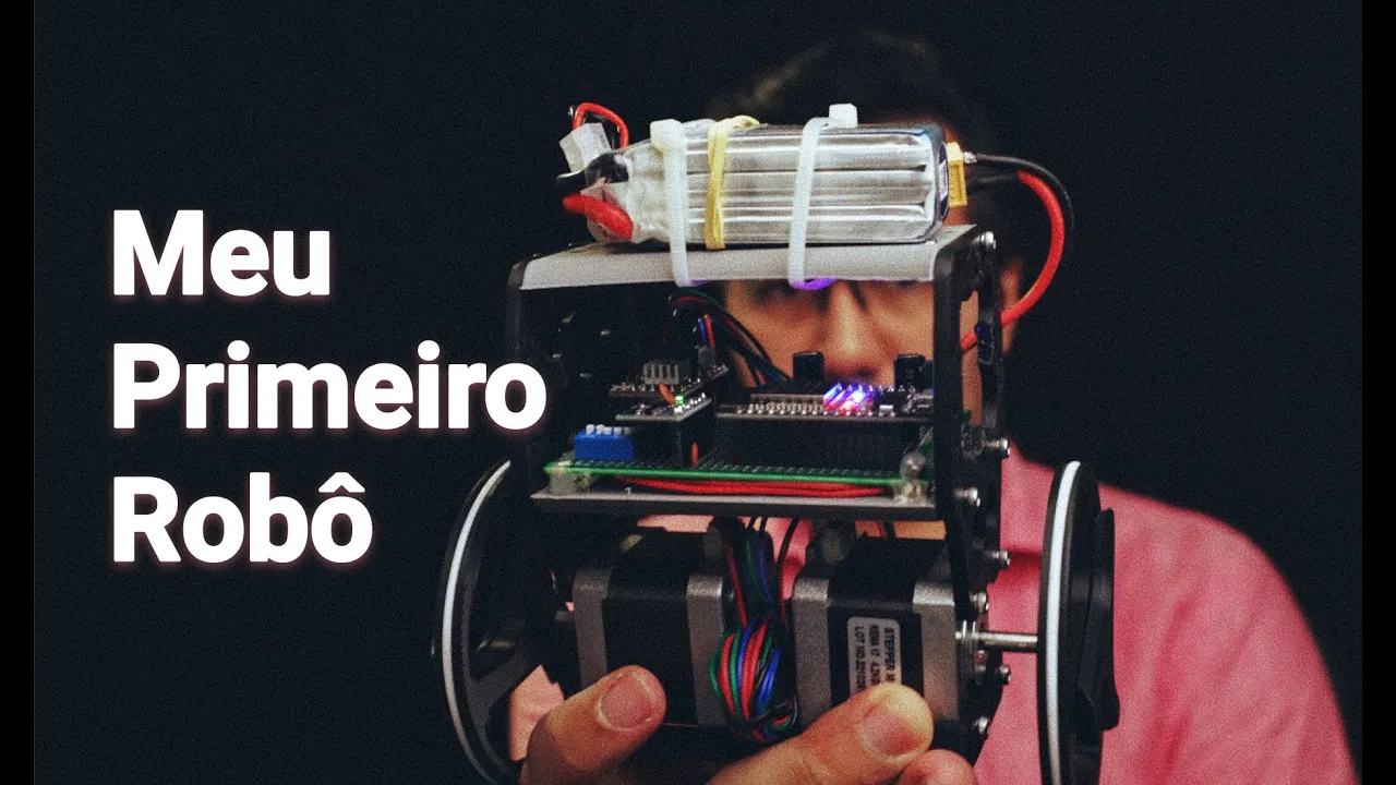
A self-balancing robot maintains equilibrium by using an inverted pendulum principle, where the center of mass must stay aligned above the wheels; this is achieved through a PID (Proportional-Integral-Derivative) control algorithm that continuously measures the robot's angle using a gyroscope/accelerometer sensor (MPU6050) and adjusts motor speed accordingly to counteract any inclination, with the proportional term providing immediate response to angle error, the integral term accumulating past errors to correct persistent biases, and the derivative term anticipating future changes to reduce oscillations.
Click to watch →
Sensor Fusion
Sensor Fusion
0:07- 1
Demonstrates MPU 6050 IMU with accelerometer and gyroscope wired to Arduino.
- 2
Shows raw sensor outputs: jittery accelerometer and drifting gyroscope data.
- 3
Highlights complementary filter for smooth, accurate orientation tracking.
Kalman Filtering and Advanced State Estimation Algorithms
While complementary filters are popular in beginner Arduino projects due to their simplicity and low computational overhead, they suffer from significant limitations in dynamic environments. A complementary filter relies on a fixed, hand-tuned weight (gain) to merge gyroscope and accelerometer data. This rigid approach struggles to handle vibration, translational acceleration, and rapid, erratic movements, which introduce orientation errors. To overcome these limitations, advanced applications utilize Kalman Filters (specifically Extended Kalman Filters) or Madgwick/Mahony algorithms. The Kalman Filter dynamically estimates the optimal state by modeling system and sensor noise in real-time, providing vastly superior accuracy in highly dynamic conditions at the expense of computational complexity. Alternatively, the Madgwick filter uses a gradient descent algorithm that delivers Kalman-like accuracy with computational efficiency near that of a complementary filter, making it a highly effective alternative for resource-constrained microcontrollers tracking complex motions.
Basic understanding of IMU sensors, specifically the operational differences between an accelerometer (measures gravity and linear acceleration, prone to noise) and a gyroscope (measures angular velocity, prone to integration drift).
Fundamentals of Arduino programming, including reading sensor registers over I2C communication and working with basic data structures.
Basic trigonometry and coordinate geometry concepts, particularly understanding Euler angles (pitch, roll, and yaw) and using trigonometric functions like arctangent to calculate tilt.
Elementary familiarity with the Processing development environment and Serial communication protocols to stream data between hardware and software.
Implementation of advanced state estimation and data fusion algorithms, such as the Kalman Filter or Extended Kalman Filter (EKF), for superior noise rejection.
Transitioning from Euler angles to Quaternions for 3D orientation representation to prevent mathematical singularities like gimbal lock.
Integrating a magnetometer (upgrading to a 9-DoF system) to calculate an absolute heading/yaw and implementing Madgwick or Mahony filters.
Applying filtered orientation data to closed-loop control systems, such as PID-controlled self-balancing robots, active camera gimbals, or drone flight controllers.
174.2K views1.4Klikes2:07@geekmomprojectsOriginal Release: 2013-04-02
This is the MPU 650 IMU. It contains a threeaxis accelerometer and a threeaxis gyroscope.
And as you can see, we have wired it to an Arduino Uno, which sends the signals from the accelerometer and the gyroscope via the serial port where they're received by this processing sketch that displays with a yellow rectangle data from the gyroscope. This blue rectangle shows data from the accelerometer.
And this green rectangle shows a combined version of the two via a complimentary filter. And you can see as we rotate the IMU about the X ais and about the Y ais, we didn't program in the Z-axis, but you can see that the rectangles follow the rotation, but the sensors are sensitive to the rotation in different ways. The accelerometer rectangle, the blue one in the middle, is very jittery and it's sensitive to any acceleration I give it as I rotate it. And you can see that the gyroscope data has started to drift. I can lay the IMU flat, but the gyroscope uh is systematically off. And the more I rotate it, the bigger the error will get. Now, as I do this, you see the gyroscope is off and accelerometer very sensitive to disturbances. But the filtered data that combines the accelerometer and gyroscope data is much smoother than the accelerometer and far more accurate than the drifting gyroscope data. And that is a demonstration of using a complimentary filter to combine gyroscope and accelerometer data.
Up Next
11:00
Complementary Filter for IMU Sensor Fusion | Lesson 11
@dianewilliams5830
4.3K views•2020-03-25

58:25
MathWorks Virtual RoboSub Simulation Environment | Webinar 2026
@RoboNationInc
209 views•2026-03-10

11:04
How to Build a Self-Balancing Robot: Arduino Nano & MPU6050
@easytechzones
16.8K views•2022-03-09
25:22
Micromouse: The Fastest Maze-Solving Robots on Earth
@veritasium
23.5M views•2023-05-24
Related Study Plans & Knowledge Roadmaps
Structured learning paths in Robotics
robotics
Building Delta Robots: Kinematics & Pico
01Foundations of Delta Robots & Mechanical Design
02Electronics and Microcontroller Setup with Pi Pico
03Delta Robot Kinematics and Coordinate Math
+ 3 more learning modules
65h6 modules
Explore Roadmap
robotics
Building Ballbots: Dynamics, Kalman & LQR
01Embedded Electronics & Omniwheel Actuation
02Ballbot Kinematics & Rigid Body Dynamics
03IMU Sensors & Kalman Filter State Estimation
+ 2 more learning modules
42h5 modules
Explore Roadmap
robotics
Micromouse: Hardware, PID Control & Flood-Fill
01Electronics & Teensy Microcontroller Basics
02Sensors and Actuators: Motors, Encoders & IR
03Precision Movement: Implementing PID Control
+ 2 more learning modules
35h5 modules
Explore Roadmap
robotics
CDPR: Kinematics, Arduino & Winch Control
01Foundations of Arduino & Basic Electronics
02Stepper Motors and Winch Mechanics
03Kinematics of 2D Cable-Driven Robots
+ 2 more learning modules
28h5 modules
Explore Roadmap