Ligand Field Theory Explained: Bonding & Magnetism

[00:00:18]Good evening everybody. Today, we will just slowly moved to the ligand field theory. So, how the ligands around the different metal centers can give rise to a typical field which is completely different from the crystal field. But before proceeding to that particular theory, how we can utilize that theory to explain some of the bonding parameter for the different metal complexes. We will finish the remaining part of the magnetic properties, what we are talking about that because these magnetic properties or magnetic behavior for the different metal complexes are basically supporting our corresponding proposition for crystal field theory. That whatever ligand we have which is surrounding the metal center, and if metal is there as M n plus, and if we can have say 6 ligands. So, without considering the corresponding bonding parameter between M and the different ligand and the ligand donor atoms, we can talk about the corresponding orbitals which are occupying the different number of unpaired electrons. So, these unpaired electrons are giving rise to very interesting properties for these metal complexes when they are isolated as a mononuclear compound, if they are present in a dinuclear compound, which we will see further again when we will be talking about little this things in terms of the corresponding biological aspects of metal complexes, that in different biological systems we can have several paramagnetic centers, and those paramagnetic centers can bind some other small molecules which are very useful in our system for our living or different living organisms, such as O 2 molecule which itself is also paramagnetic. So, the situation is becoming much more complex, when 2 metal centers are there, having some amount of paramagnetism, it can be 1 electron paramagnetism or it can be 2 electron or 3 electron paramagnetics. And apart from that, the small molecule or small group which is bound to these metal centers, are also paramagnetic in nature.

[00:03:08]So, overall, how we can monitor experimentally the corresponding behavior? So, what experiment we basically propose for finding out that particular properties of these centers. So, in that individual centers for the individual paramagnetism as well as the overall some interaction, such as in some case it can be anti ferromagnetic or in some other cases ferromagnetic.

[00:03:39]So, we will see that, what are the different experimental evidences? How we can measure this magnetic movement, because theoretically already we have seen that there are several techniques what we can use for, say, different types of interactions, whether we are involving the corresponding mu J equation, mu L equation or mu S equation to determine the corresponding magnetic moments and their orbital contributions also.

[00:04:09]But, right now what we can see that, we want to measure the corresponding magnetic susceptibility.

[00:04:14]So, it is the kai N values, which we are going to measure to find the exact number of unpaired electrons which are present in a particular metal complex or any other multi nuclear metal complex also. And the paramagnetic substances which are present there, if will place them in a typical magnetic field, they will be attracted. So, how we can measure this amount of attraction between the paramagnetic centers, that means, the between this paramagnetic compound and some applied magnetic field, that will find out. Because all the different other spectroscopic techniques which are depending on magnetic field can also give some idea, whether we should be able to measure this particular paramagnetic substances for those spectroscopic signatures, like N M R and E P R using those magnetic fields. So, the first thing what we can use, is a very simple thing that is a balance; analytical balance which is very much sensitive, say up to say fifth place of decimal we can measure. So, that balance, it can be converted to a Gouy balance, where we use some permanent magnet; and within the magnetic field we place the corresponding sample and we measure the weight. So, use of this Gouy balance takes the weight change of the sample; that means, the change of weight in presence of the magnetic field and in absence of that magnetic field. So, we will use the analytical balance. And the sample is placed in a homogeneous constant magnetic field, so of a very little bit of high magnetic field value of, say, 1 tesla to 10 tesla. And, whatever measurements we make, it can be calibrated against a known standard like mercury cobalt II tetrathiocynate compound; tetrathiocyanate compound of this cobalt, so which has a fixed magnetic movement value as well as the corresponding molar magnetic susceptibility, that means, the kai n value. Also, we can use copper sulphate penta hydrate also, so we can use copper sulphate pentahydrate. In these 2 samples, these are very good standards for measuring the mu effective value, or mu spin only value. Because, in this particular case, what we know that, it has one unpaired electron and theoretically we can get the corresponding mu effective or mu spin only value for this copper sulphate sample; but also we can have some value for this corresponding molar susceptibility or gram susceptibility values. So, which are simply compare the corresponding kai g and kai n values when we take certain amount of this copper sulphate solution; and in an uniform measuring technique, that means, we take the corresponding tube which is known as the Gouy tube. And, these Gouy tube is there and which is one, once it is filled with the standard sample and we take the 2 weights; that means, one weight in absence of the magnetic field and one in presence of the magnetic field.

[00:07:59]Similarly, the same tube can be filled with the, next time can be filled with the sample. So, this is for standard; and this is for the sample itself, and there also we have 2 weights W 1, W 2 or rather we can consider it as W 3 or W 4. So, using these 4 weights - W 1, W 2, W 3 and W 4, and by knowing the corresponding kai g values for this copper sulphate, we can determine the corresponding mu effective value or the mu spin only value for the unknown sample what we are going to measure in the solid state in the powder form. So, this particular technique is useful for solid powdered sample. We cannot go for anything which is in solution or some other thing, when we measure the corresponding biological samples which are always present in solution.

[00:09:07]So, for those samples we have to use some other different technique, where the sensitivity of the corresponding balance is much more. And, we can sense one particular metal center, say, if it is hemoglobin or myoglobin within a very big protein envelope. So, protein chain is there, which has a very high molecular weight, several 1000 kilodalton; and we have to sense this particular paramagnetism which is trapped inside the macro molecular chain of the protein structure.

[00:09:43]So, the sensitivity of their corresponding balance should be much more, such that we can sense the corresponding values of this small chain, in the corresponding kai g or the kai n values. So, this standard is very much useful for any other thing; that the standard can be utilized to calibrate the instrument, that means, the same tube, where we can go for the corresponding diamagnetic correction for the tube also.

[00:10:11]For, from the known Pascal’s constant constants, we go for the corresponding diamagnetic correction and measure ultimately the mu effective and its corrected form.

[00:10:22]So, it basically measure; the Gouy balance what we can have, is used to measure the magnetic susceptibility, that means, the kai g. And which when multiplied by the molecular weight, we get the corresponding kai n value.

[00:10:37]It was first invented by Louis Georges Gouy. So, this, that is why it is name as Gouy balance; is very simple technique and very useful technique, where we have the permanent magnet. So, these are the 2 poles of the permanent magnet. And we place the sample within a tube which is known as the Gouy tube. And magnet, one it is switched on and another case it is switched off. And this the lower end of a balance which can be a single pan balance, which can measure up to fifth place of decimal, which is a very sophisticated magnetic balance, and which is encased in a glass field.

[00:11:20]And this particular sample which is facing this magnet, it has to be seen, there it is extending because the tube is big one. So, it is the only drawback of this particular technique, is that we can use up to say 8 to 9 centimeter of this length; and for that purpose if the tube is not very much big, is close to that of our NMR or EPR tube. And the magnetic field is extended; this is the maximum possible magnetic field where we are getting at the center of the magnet and which is extending from 1 to 0. So, this, here we do not have this magnetic, any kind of magnetic field.

[00:12:03]So, this, because we have to go for the corresponding integration from A 1 to 0; that means, maximum possible magnetic field to A 0 magnetic field situation; and in that situation, we just use to measure the corresponding change in the weight. That is why we require comparatively large amount of sample which has to be filled this tube, and the tube is placed inside the magnetic field. So, we get some attraction and repulsion when we have the diamagnetic sample. The diamagnetic samples get repulsion by the magnetic field. And when we have a metal complex, and even it is bound by several such ligand centers and if the ligands are very big, and is also, it can have this several steric crowding, and it can have several other atoms. So, this ligand part is also diamagnetic. So, within a diamagnetic host or diamagnetic envelope, we just simply go for the measurement of this corresponding paramagnetism which is originating from the metal center for the complex.

[00:13:25]So, for that also one is tube, the tube what we are used for measuring and two is the ligand part. These two, we have to use for the diamagnetic corrections; and for that standard tables are there and which are Pascal’s constants, and those Pascal’s constants are used to go for this corresponding corrected kai n and the kai g value, to determine the corresponding mew effective value after this correction is known as the mu effective corrected one. So, within the magnetic field, when we place the sample, there will be a change in apparent weight of the sample, when the magnetic field is turned on. So, that is the basic principle behind this simple technique of Gouy balance, for measuring the paramagnetism of these metal complexes.

[00:14:36]But, what we can use nowadays, to see very small magnetic interactions when we have multi nuclear metal complexes, such as 4 copper centers are present in any sample, or any biological sample such as hemocyanin or any other thing; but 2 copper centers are present and sometimes we have the corresponding ambiguity, whether the copper irons present in hemocyanin molecules are paramagnetic or not; that means, whether the copper centers present are in plus 2 oxidation state which are in only big paramagnetic, or in its reduced form, that means, the copper 1 plus, because the q plus state, it will be diamagnetic. So, for that very sensitive magnetometer we require, utilizing the super conducting quantum interference technique or interference device, the squid is useful for that particular purpose, to measure very low magnetic movement value. And when, it can be used for any change for the variable temperature measurements also, for knowing the ferromagnetic behavior or anti ferromagnetic behavior at very low temperatures.

[00:15:48]So, this is another schematics, which basically tells us that, how the thing is basically changing; that means, this length is extending from a maximum magnetic field possible to A 0 magnetic field. But when it is attracted by the magnetic field, we see there is a change in the weight; that means, the tube goes inside the magnet, when the magnet is turned on. So, sample is basically packed nicely; uniform packing is required for this tube. And it is placed in a glass tube, very simple glass tube. Homemade glass blowing section can also do that Gouy tube for us.

[00:16:33]And, electromagnet, this end, not a very sophisticated one; the permanent electromagnet we need which is providing the corresponding magnetic field. So, by doing this, we just basically, change of weight can be measured using this balance. So, is a single pan, good balance is required. So, balance, from the balance pan we put the hook, one hook, and from that hook, basically, it is suspended within the magnetic field.

[00:17:04]So, the next particular balance what we can use, is a different one, compared to the very simple Gouy balance, which is known as Evans balance. So, in this particular technique, the balance is a different one, where we can consider it as a torsion balance, is not is in simple single pan balance what we use from certain good companies like metlar and others where a single pan balance is very much useful to measure any quantitative determination of weight change upto fourth or fifth place of decimal. So, in this torsion balance, a sample is placed in a fixed position, and a variable secondary magnet is utilized to bring the magnet back to its initial position. That means, we just use the corresponding magnetic field, the delta h can be added to the h, to bring back the magnet to its original position. And this particular torsion balance is particularly useful for different types of susceptibility balances. So, these balances are known as susceptometers or susceptibility balances, where the technique for this measurement is different from that of our Gouy balance.

[00:18:20]And, third type of the balance what we can have, the corresponding Faraday balance. And here, the sample is placed in a magnetic field of constant gradient, and the weight is taken on a torsion balance. So, balance utilized it is a torsion balance. And the method can also provide on magnetic anisotropy. That means, if the magnet is not behaving uniformly in its 3 directions, 3 anisotropy directions like these x, y and z. If the magnetic field is different from one other axis, compared to x axis or compared to the y axis, then we can have the corresponding magnetic anisotropy present in the sample.

[00:19:08]And that anisotropy gives us very important information’s related to the corresponding magnetic interactions, for the corresponding interactions, giving rise to the 2 paramagnetic centers which are interacting. So, what we do in Faraday balance? The field is completely different, because the pole heads are different which is providing us some inhomogeneous magnetic field. In case of Gouy balance, we have a homogeneous field, and uniformly the tube is extending from the center of the magnet to outside of the magnet field. The pole pieces here, in case of this Faraday balance are so created, that there is a region in which the product of the field strength and the field gradient is in the z direction is constant. That means, on the upward direction we are not changing the corresponding product of field strength and field gradient; that means, with the change in the distance from the center of the magnet, this particular product in the z direction are not changing, and sample is basically placed in that area only. But in case of Gouy balance that is changing uniformly, as we move from a center of the magnet to outside. So, this homogeneity is created for that reason only, such that the field gradient and the field strength remain constant, along the axis, where we are taking the corresponding weight in, say, z direction. The force which is being operating on the sample, is experiencing that particular force is independent of the packing of the sample. That means, in case of Gouy balance we need some uniform packing of the sample and which is nicely packed. But in this particular case, if we do not pack in a uniform way, there is no harm for the measurement, but it depends only on the total mass of the material which is present in the system. And what are the difficult, at typical advantages for this method, over the gouy method, or the corresponding susceptibility torsion balance method is that, the method is sensitive highly reproduceable; that means, if we have 10 measurements and all the measurements would be pretty close to each other. So, there is no need to take the average of, say, 3, 4, or 5 measurements. So, this is sensitive and highly reproduceable, and can be applied to also to the single crystals. Since, we are talking about the magnetic anisotropy, and if we place the single crystals, along the corresponding crystal axis x, y and z, so we can differentiate the corresponding magnetic movement values in different axis; that means, mu x, mu y and mu z values, which we can find out if we go for the corresponding measurement using a single crystal.

[00:22:18]The force, here again is measured as a weight change, using now again a torsion balance.

[00:22:23]So, balance is again a torsion balance, but only difference from the torsion balance for the measurement of the susceptibility balance which is that, the magnet is inhomogeneous, and which is focused for measuring the corresponding magnetic anisotropy.

[00:22:39]So, if we go for this thing that how we are going to measure the corresponding magnetic moments? And the magnetic moments are very much useful for knowing the corresponding crystal field theory.

[00:22:54]So, basically, all these measurements are basically supporting our crystal field theory, where we have seen that the corresponding number of electrons, if we, say, a nickel compound in plus 2 oxidation state, or some binuclear nickel compound, which is binuclear. So, we can measure in both these 2 cases, the corresponding mu effective values and here also mu effective values.

[00:23:46]And we just try to look at, how these 2 paramagnetic centers; obviously, these 2 nickel are paramagnetic in nature, because we have 8 electrons giving 2 unpaired electrons in the e g level. And the corresponding spitting for this nickel in octahedral geometry, these 2 are also in octahedral geometry. And, in biological sample, it is also present like this, in ureases. So, in urease molecule, we find the 2 nickel centers are there, which is responsible for urea hydrolysis; urea is nothing but this. So, this is getting hydrolyzed. So, that can be studied, when 2 nickel centers are in close proximity, at a distance of, say, 3 Armstrong, which is basically binding the urea molecule. And that urea molecule is undergoing the hydrolysis through some nucleophilic attack by H O minus, or H 2 O. So, nucleophilic attack of H O minus or H 2 O can lead to the catalytic reaction.

[00:25:12]But, all these catalytic reactions what we are talking about, is taking place on this 2 nickel substrates. So, it is basically, this is the platform. And on that platform the urea is coming and binding to these centers. But if we talk in terms of the corresponding mu effective values for these 2 centers, so that these 2 centers are ferro magnetically interacting or anti ferromagnetic interacting or that can have some effect on the hydrolytic potential of the urea molecule for the different ureases, that we can see that, simply by looking at the corresponding crystal field theory, without knowing the bonding parameters, how these bonds are forming, and what are the corresponding nature of the corresponding metal ligand bonds, we can talk in terms of the number of unpaired electrons present on the nickel center. And, how the 2 unpaired electron from the first nickel center, which we can also consider as nickel A and the nickel B, the second one; and how they are interacting, that can also be very nicely explained or determined, in terms of the corresponding crystal field theory. Because this theory tells us that, we are not focusing much attention on the ligand charges or the point charges or the different dipoles, which are surrounding this particular metal centers.

[00:26:44]So, we are not talking anything related to the corresponding nature of this bonding with this nickel center, for the different ligand donor atoms. So, crystal field theory therefore, only focusing our attention, or taking us to consider this ligands as only to point charge or the dipole, dipole only; and does not take into account, the overlap of the ligand and the metal orbitals. So, these are basically the limitations of the crystal field theory, where we are not considering any kind of overlap of ligand and the metal orbitals. So, that basically gives us some idea that, when we talk this in terms of the crystal field theory, and considering the ligands as point charge or the dipole only, what we see that, we are not considering any kind of overlap between the metal and the ligand orbitals. So, if we have 2 centers, such as, this 2 can be nickel 2 or copper 2. So, when these are bound; so in this particular case, in case of urease, it is bound by a carbamate unit. So, if we consider that we have 2 unpaired electron on the first copper and 2 other on the second copper, and if we think of the interaction which can be, say, ferromagnetic, that means, we are adding of the magnetic movement from one copper center to the other. But we should have something to consider.

[00:28:38]Also, that interaction of ligand orbitals to the metal orbitals, that we are neglecting in case of crystal field theory.

[00:28:49]So, if the super exchange is taking place through the bridging ligand for this corresponding magnetic behavior, whether it is ferromagnetic in nature or anti ferromagnetic in nature, we should consider the overlap of the orbitals of M and L. So, we should consider the overlap. But which we are not getting from the crystal field theory, that is why, this is the typical limitation of the crystal field theory. And we should modify this particular theory for considering this particular overlap. And also when we fail to explain the nature of the carbon monoxide ligand as we see in the spectrochemical series that carbon monoxide is a stronger ligand than cyanide ion. In several such complexes, that when we consider the nickel tetracarbonyl ion, ion pentacarbonyl or chromium hexacarbonyl, we in all these cases we see that carbon monoxide is behaving as a very strong ligand compared to its CN minus analog, and this complexe is having metal in low oxidation state. So, in several, that these complexes where the oxidation state of the metallic is 0, or in the low oxidation state, where unable to explain in terms of the crystal field theory, why CO is stronger than CN minus, which is a neutral ligand. So, that also compel us to consider that there is certain amount of overlap between the carbon monoxide orbitals; that means, the formation of the corresponding carbon monoxide molecular orbitals should, we should have. And these carbon monoxide molecular orbitals, if we interact with the ligand d orbitals, to give us some good information about the metal and ligand overlap.

[00:30:49]So, we propose the theory which is termed as a ligand field theory, which basically, all the time will be utilizing the corresponding molecular orbital approach, as we see for the simple molecule. And this approach, what we see that, if we just consider that our ligand is carbon monoxide; that means, the carbon monoxide is forming from carbon and oxygen. So, instead of considering the carbon monoxide as a point charge or dipole, we will consider the corresponding molecular orbitals of the carbon monoxide. And these carbon monoxide ligands we can use as utilizing their hybrid orbitals or the pure s orbital, which are pointing towards the metal 2, 4, the corresponding sigma bonds to the metal.

[00:31:40]So, today, we just simply start our discussion by considering that only sigma bonds are forming between metal and ligand, where the theory can be considered as a ligand field theory, which is basically admixture of molecular orbitals of the ligand and the corresponding pure orbitals or hybrid orbitals of the metal center, giving rise to the different orientation of the different bonding as well as anti bonding orbitals. So, arrangements of these orbitals in different energies, and their corresponding occupancy for the unpaired electrons will tell us the corresponding theory as the ligand field theory.

[00:32:25]And, what we have ignored in crystal field theory, that the nature of the ligands. Slowly we will just go towards this theory that, now we have to consider the nature of the ligand, whether the ligand is carbon monoxide or CN minus or M 3 minus or S N minus. So, they all have different types of hybrid orbitals available for donation to the metal center. Since, we have ignored this nature of this ligand, we are unable to explain in terms of crystal field theory, the corresponding spectrochemical series; that means, why some ligands are in the, strong field ligands and others are weak field ligands, so though the interaction is not purely electro static in nature.

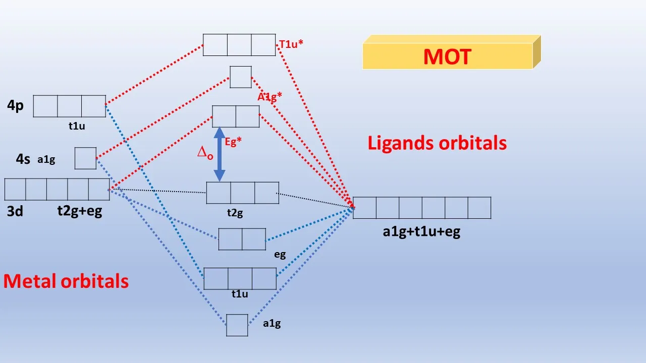
[00:33:14]So, we just use the typical molecular orbital theory; what we know so far for simple molecule, simple covalent molecules, like carbon monoxide, like cyanide, like thiocyanate, like azeite, will utilize that molecular orbital theory for the, getting the corresponding LFT or ligand field theory. Now, we have the different valence orbitals on the metal and ligand are used to form the different SALCs; SALCs are nothing but symmetry adapted linear combination.

[00:33:54]So, we have now, the different SALCs. So, this is nothing but we are talking with the symmetry which is very important; that means, whether we are talking a corresponding metal complex. So, that is why we are talking so much about the symmetry of the metal complex, whether it is tetrahedral, whether it is octahedral, or square pyramidal, or trigonal bipyramidal. So, those symmetries are very important, because those symmetries will dictate that corresponding adaptations. So, it is symmetry adapted linear, the combination is only linear combinations. So, symmetry adapted linear combinations of the different orbitals. So, if we have those orbitals; so symmetry will dictate a particular type of linear combination, and that combination will give us; these are our new molecular orbitals for the complex. So, if they are coming out from the ligands, we have symmetry adapted linear combinations of those orbitals coming from the ligand. And also, from the metal center, we are having large number of other orbitals, say, s orbital, p orbital, and the d orbitals. So, this s, p, and the d orbitals can form also some amount of symmetry related molecular orbitals for good overlap with the ligand orbitals. So, we will be utilizing this valence orbitals as the different SALCs. And then we will utilize the preliminary energy level diagram and overlap consideration for knowing the relative energies of the molecular orbitals for their estimated form. That means, whether the energy is higher or lower, that we will just simply guess from these combinations; that means, whatever we are getting, whether we are getting some as bonding orbital or some as the corresponding anti bonding orbital. So, two types of bonding we will consider in this particular theory. One is the typical sigma bonding, which is sometime very close to that of our crystal field theory, when these interactions were purely electrostatic, but now will have direct overlap between the metal and ligand orbital. And if there is a head on overlap, we will be talking in terms of the corresponding sigma bonding and the ligand has a single balance orbital. So, if we have some sigma bonding orbitals available on the metal center, so ligands will have some symmetry related combinations of the different orbitals available on the ligand or sometime the pure orbital, say, p orbital; the p orbital which can be considered as the valence orbital, and which is directed towards the central metal atom to give us the corresponding overlap for sigma bonding. Similarly, what can happen for our pi bonding also. So, we will get the typical pi bonding also, because this pi bonding can now modify the corresponding nature of this metal ligand interaction differently. So, that is why we are getting this information, that why carbon monoxide is a stronger ligand than cyanide. So, when the ligand has a field orbital of pi symmetry, which is important. So far, we are not considering anything related to, that the ligand field orbital of pi symmetry we are not considering.

[00:38:00]So, if it has a field orbital of pi symmetry around the M L axis, so those electron density can be donated to the metal, and we can have the corresponding metal ligand pi bond. So, not only sigma bond which can be considered as a single bond, we can have a multiple bonding between the metal and ligand to give rise to some kind of pi bonding also, like the formation of ethylene and acetylene; that means, the multiple bond is also permissible for these system, where we can have both sigma as well as pi bond.

[00:38:36]So, these are the 2 pictorial representations which typically tells us that how sigma bonding can take place, where the metal orbital which is the typical d z square orbital having 2 lopes directing towards the z axis, along the z axis. So, if the ligands are approaching along the z axis, we find a head on overlap between the metal d z square orbital and the ligand p z orbitals. So, these are the ligands p z orbitals. These ligands p z orbitals are also facing the z direction.

[00:39:15]So, that is why, we will have good overlap with a ligands p z orbitals, with that of the metal d z square orbitals.

[00:39:23]So, the metal d z square orbital which we have seen in case of the corresponding magnetic movement in the spectroscopic term, that they are basically, sometime they are not contributing much towards the corresponding magnetic movement, but when we are considering the sigma bond, they have the typical sigma symmetry. That means, the orbitals, the e g set of orbitals in OH symmetry have the matching sigma symmetry with respect to the overlap with the p z orbitals of the ligands. So, if the ligand along the z axis for an octahedral symmetry, so along this direction we have 2 ligands.

[00:40:09]So, these 2 ligands will nicely overlap with the metal d z square orbitals to give us sigma bonds.

[00:40:19]Similarly, the x square minus y square orbital also having, coming from the same e g level or the metal center in the OH symmetry. So, these orbital, these 2 orbitals are also nicely giving us the corresponding sigma overlap. So, even they are in x square minus y square symmetry. So, they also go for some head on overlap with the ligands coming from x and y direction. So, these 2 orbitals are well matched for giving us the corresponding sigma symmetry for the formation of the sigma bonds to the metal complex in octahedral symmetry.

[00:41:03]So, utilizing this ligand field theory, we describe the bonding, the orbital arrangement; that means, how many of them are bonding orbitals, and how many they are anti bonding orbitals, and what are the corresponding separation between these orbitals, and whether those are matching for the corresponding spectrochemical series, that can be obtained from this theory, which are therefore characteristic; that the bonding parameter and orbital arrangement thing, which are characteristic for the all the different types of coordination complexes. And now, if we having 6 ligands around the metal complex in octahedral geometry we will have 6 sigma bonds, facing to each from the 3 axis x, y and z. So, the 6 sigma donor ligands, how they are forming, because the molecule orbitals will be formed, like coordination result from the donation of 2 electrons by each of the 6 sigma donor ligands.

[00:42:04]So, if we have 6 sigma donor ligands along the 6 axis of the octahedron to the d orbitals on the metal ion, we find that in case of octahedral complexes the ligands will approach along the x and y and z axis. And the sigma symmetry orbitals for bonding and anti bonding combinations with the d z square and d x square minus y square orbitals only, because these 2 orbitals are only pointing towards the 3 axis. So, if the combination is there for sigma symmetry, we will have sigma bonding as well as sigma star which can be considered as the anti bonding level. So, these 2 orbitals will be utilized for the bond, sigma bonding for these metal complexes in OH symmetry. But, what about the T 2 g set? The T 2 g sets of the orbital, that means, the d x y, d x z and d y z orbitals will remain as non bonding orbitals, because they are not facing directly to the ligand systems, that means, the ligand orbitals. They will not have any interaction with the ligand orbitals. And some weak bonding or anti bonding interactions can take place with the s and the p orbitals of the metal ion. And we will have a total of 6 bonding and 6 anti bonding molecular orbitals. So, we will have non bonding orbitals. And then we can have the corresponding involving the s and p orbitals.

[00:43:49]So, we will have 1 is 3 p. So, 4 orbitals and plus 5 of the d orbitals. So, all these d orbitals can give rise to the corresponding 6 bonding and 6 anti bonding molecular orbitals for the system.

[00:44:04]So, what we get? That 6 ligand donor orbitals collectively form a reducible representation.

[00:44:11]So, since, we are talking the corresponding symmetry level. So, for getting all these things, we have to utilize the corresponding corrected table for the symmetry level of the different orbitals. So, if we just utilize a corresponding corrected table for octahedral symmetry, we will have the typical reducible representation. So, we all know, from the, this corresponding thing that what we get for this particular arrangement, that if we get the corresponding corrected table for octahedral symmetry, the reducible representation of this octahedral symmetry we can get. And from that reducible representation, we can have the corresponding irreducible format, that means the irreducible representation.

[00:45:08]And those irreducible representations are some symmetry level. And from those symmetry levels we will take out the corresponding orbitals for the matched one. So, the 6 ligand sigma orbitals, the p orbitals or the hybrid orbitals with the same symmetry can match; that means, the 6 SALCs from the ligand. So, either s and p orbitals or the hybrid orbitals from those ligands, will, can match the symmetries of s p x, p y, p z, and 3 d z square, and 3 d x square minus y square metal orbitals. So, matching will be with all the orbitals. So, now, we will find slowly, that whatever we are discussing for crystal field theory, we are just talking in terms of the corresponding d orbitals only, but now we see that s and p orbitals can also show some contribution for the formation on these regular orbitals. So, the combination of the ligand and metal orbitals forming 6 bonding and 6 anti bonding orbitals with a 1 g, e g and t 1 u symmetry. So, these are the 3 irreducible representations which will be coming out from the corresponding reducible representations, for the corresponding corrected table. And these are the corresponding sets which are the corresponding symmetry level for those orbitals. So, 6 bonding orbitals are filled by electrons donated by the ligands. So, whatever bonding orbitals we will have, so those bonding orbitals will be occupied by the ligand electrons, which are donated to the metal centers.

[00:46:54]So, the metal T 2 g orbitals; so these are the corresponding a 1 g, e g and t 1 u set, but the T 2 g orbitals, which we all know, that the T 2 g set and e g set. So, this is the corresponding spectroscopic level, and the orbitals will be leveled in the small lower case t 2 g. For these orbitals do not have appropriate symmetry, that is why we are talking that these 2 orbitals are remaining as the corresponding non bonding orbitals.

[00:47:26]So, the molecular symmetry terms, the 6 lone pair orbitals from the ligands, one from each from the 6 symmetry adapted linear combination, that we are just now discussed. And also, sometimes we are considering these as ligand group orbitals. So, if the ligand is providing 6 such groups of orbitals, and the combination of those will be considered as the ligand group orbitals or SALCs. So, these are the corresponding irreducible representations from the reducible representations; the gamma red, it can be represented as the corresponding irreducible representation. And this basically span these 3 symmetry levels, A 1 g, T 1 u and E g.

[00:48:17]So, our orbitals, the SALCs or L G Os will have these symmetry levels for the molecular orbital formation. So, this is the reducible representation for the octahedral symmetry. And these are the all possible symmetry operations and their contributions for the reducible representations. And there are several useful techniques for getting the corresponding irreducible representation from the reducible representation, for any such table for this representation.

[00:48:51]So, this reducible representation will reduce into A 1 g, E g and T 1 u. So, this gamma or sigma will give rise this 3 levels.

[00:49:02]And we will now locate this 3 types of symmetry levels for those orbitals, for the different sets of orbitals which are coming from the symmetry levels.

[00:49:14]So, if we have the metal s orbital, which is symmetric; and the 6 ligands are approaching along the 6 axis; and along these 6 axis we have the corresponding symmetry which is spherically symmetric. So, this we can level as a 1 g symmetry; and this a 1 g symmetry which can match very well if we can put the ligand also. The green balls are the corresponding ligand orbital; either they are the hybridized orbitals or the p o p orbitals, the lopes from the p o p orbitals.

[00:49:55]So, they are basically overlapping with these, which is a spherically symmetric arrangement. So, we have the match ligand orbitals with the match metal orbital with a 1 g symmetry. So, a 1 g group orbitals. So, these we call at the ligand group orbital, the LGO’s or the SALCs. So, a 1 g group orbitals have the same symmetry as an s orbital on the central metal. So, if the central metal ion has the symmetry of a 1 g, then the ligand group orbital will definitely overlap with the a 1 g symmetry of the metal orbital. So, that gives us, for the first time, that it is completely opposite for that what we are talking in terms of the crystal field theory; that here we are just considering the symmetry level as a 1 g. And s orbital is also coming into the picture for this typical hybridization. And this s orbital can also have some overlap with the ligand orbitals of same symmetry. So, the metal also has 6 valence orbital; this is spanning; this irreducible representation. And s orbital is leveled as a 1 g. And the set of 3 p orbitals on the metal is leveled as t 1 u. And d z square and d x square can be leveled as e g. So, these are the corresponding symmetry level for all the orbitals, which are coming for the metal will take out of 5 d orbitals, we will take only the 2 d orbitals. The e g set of d orbital 3 p orbitals and the s orbital. So, 3 plus 2, 5, plus 1,6. So, these are the 6 orbitals from the metal side which will be forming the corresponding molecular orbitals to go for the overlap with the corresponding ligand orbitals. And they are nicely matching with the t 1 u set as p orbitals, and e g set for the d z square and d x s square y square orbitals; what we have discussed in detail that, these 2 types of orbitals are only utilized for sigma bond formation with the ligands.

[00:52:17]So, in octahedral complexes, therefore, the ligands approach along the x, y and z axis.

[00:52:24]So, their sigma symmetry is matching with that d z square and d x s square minus y square orbitals. And they are therefore, forming bonding and anti bonding combinations related to this d z square and d x s square minus y square orbitals from the 5 d orbitals.

[00:52:44]So, now, the ligand will also provide this particular level, that what we have shown just now; that the ligands which are approaching from the z direction. So, these 2 are basically overlapping with the d z square orbital, where the ligand is directing along the z direction. Similarly, d x square minus y square orbital from the metal is overlapping with the 4 ligand orbitals along the x and y axis. So, these 2 orbitals, the d z square and d x square minus y square can be leveled as the e g set from the metal side.

[00:53:27]Similarly, the other 2 combinations, that means, the combinations of these p orbitals from the ligand set, this is a corresponding combination from the ligand side. So, this is the corresponding combination in terms of ligand group orbitals, and these are another combination of ligand group orbitals having e g symmetry.

[00:53:50]So, what we will find? This e g group of orbitals at the same symmetry, therefore, as the d z square and d x square minus y square on the central metal. So, we will see good combination for these 2 sets of orbitals from the metal side as well as from the ligand side. And therefore, e is representation for the w degenerate level, what we all know, from the crystal field region also; that we have the e g set of orbitals are these 2, and now this is the w degenerate set. So, e g level, that means, the e g in terms of the corresponding molecular orbitals, what we will write now on the molecular orbital energy level diagram, that this e level will consider as the w degenerate level.

[00:54:41]The t 1 u group of orbital next, have the symmetry as the p orbitals on the central metal. And t therefore, represents the triply degenerate level, like the w degenerate. So, we have s orbital from the metal. We have the corresponding d orbitals, 2 d orbitals from the metal center, now the p orbitals. So, this t 1 u set, what we are getting, these are basically the corresponding p x, p y and p z orbitals. And this p x, p y and p z orbitals from the metal side what we are getting, is that; this is from the metal side, and this is from the ligand side. So, when we have, in the metal side, this orbitals are these 2, and therefore, the ligands are also providing the corresponding ends along the x axis, along the y axis and along the z axis, which are also matching with that of our t 1 u set of orbitals. So, this 3 p orbitals giving rise in these directions are basically the set of orbitals which are matching with the metal orbitals.

[00:55:54]And this ligand group orbitals are useful from this t 1 u symmetry. And those t 1 u symmetry level is the corresponding orbitals also from the metal s p orbitals, and p orbitals from the ligands, and they are utilized for the overlap. And this t 1 u set of orbitals we will find in the molecular orbital for good overlap. So, in our next class, we will find how this will just go for these overlap and these interactions. Thank you very much.