This lesson demonstrates how to test a SimpleFOC motor control system by connecting a motor to an Arduino Uno through either analog or I2C interfaces, then running test programs to verify position control, speed control, and current sensing capabilities through serial monitor feedback.
SimpleFOC Lesson 2: Basic Testing of Makerbase Motor Driver
Added:Deep Dive
Basic principles of Brushless DC (BLDC) motor operation and the core concept of Field Oriented Control (FOC).
High Performance Motor Control From the Ground Up || Field Oriented Control (FOC)
253K
Field Oriented Control (FOC) is a sophisticated motor control technique that regulates brushless motor torque by precisely controlling the current in each phase, using encoder feedback to keep the electromagnetic force vector aligned with the rotor's position for maximum efficiency; this involves converting measured phase currents into a stationary reference frame, applying PI controllers to regulate torque-producing and non-torque-producing currents, then transforming back to phase voltages and generating PWM signals through a full bridge inverter.
Click to watch →

Field Oriented Control of PMSM | شرح
1.9K
Field Oriented Control (FOC) was discovered by a German scientist in 1973 through his doctoral thesis. FOC is built on the principle of making induction motors or permanent magnet synchronous motors behave like DC motors. DC motors are easy to control because magnetic flux is always perpendicular to armature current, generating torque proportional to the product of flux and current. This perpendicular relationship is the key characteristic that makes DC motors simple to control.
Click to watch →

Unlock Better Motor Control
79K
Field Oriented Control is a fundamentally different strategy for motor control that turns two adjacent coils on and off repeatedly, trapping the magnet in a game of monkey in the middle. By carefully timing the coil pulses, FOC enables smooth motor rotation at very low speeds, solving the jitter problem inherent in basic motor control methods.
Click to watch →
Brushless DC Motors and Brushed DC Motors explained - BLDC Fan (2)
1.7M
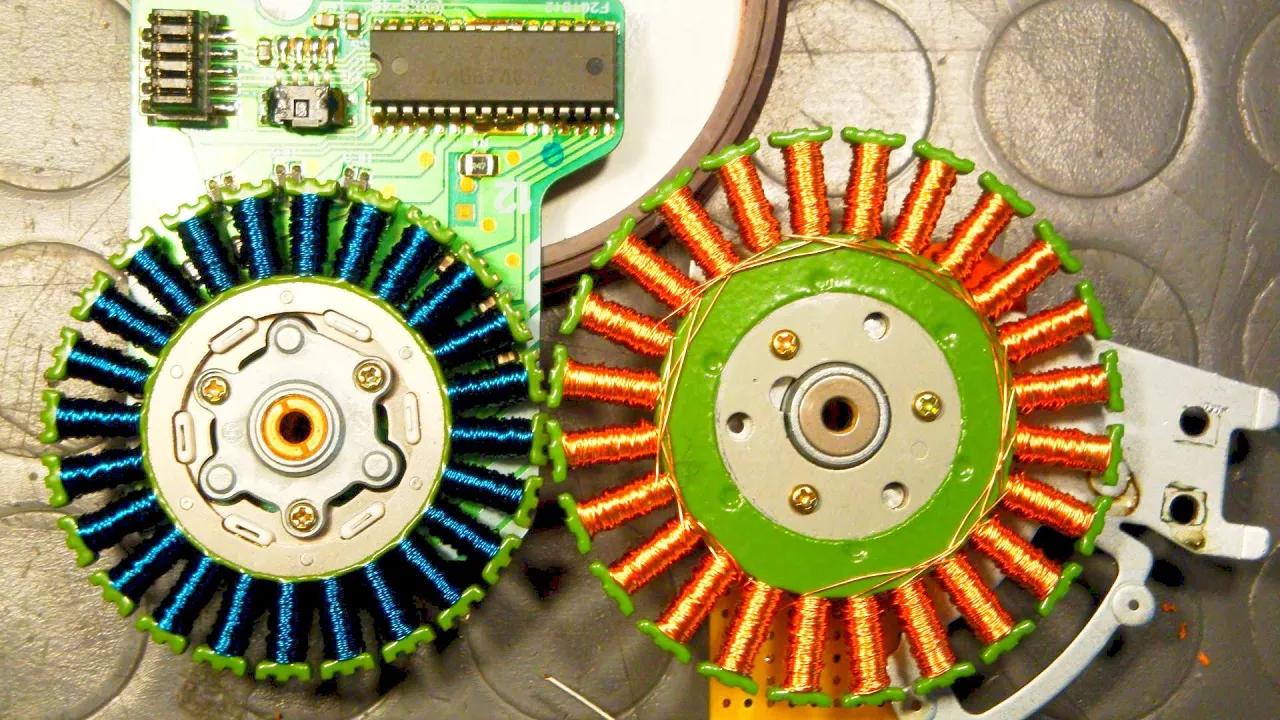
In brushless DC motors, the rotor contains permanent magnets while the stator carries electromagnetic windings. For a two-phase BLDC motor with four poles, each limb of the magnetic core carries two windings wound in opposing directions. Electronic switches (typically MOSFETs) control current flow through these windings. A hall effect sensor detects when rotor poles pass by and triggers switching to reverse the stator field direction, causing continuous rotation. This electronic commutation replaces the mechanical commutator and brushes of brushed motors.
Click to watch →

Motor Control Design with MATLAB and Simulink
129.1K
Field Oriented Control (FOC) is the fundamental concept in PMSM control that allows engineers to decouple the control of flux and torque. The core components of an FOC controller include the Park transform, current controllers, and inverse Park transform. This decoupling enables independent control of the motor's magnetic field and torque production.
Click to watch →
Deep Dive
Proficiency with the Arduino IDE, basic microcontroller programming, and interfacing with hardware pins.
Arduinoya Giriş-Sıfırdan Arduino Öğreniyorum#1
51.4K
This section teaches Arduino IDE navigation and fundamental programming concepts. The IDE includes File menu for project management, Library Manager for adding external libraries, Tools menu for board and port selection, and Serial Monitor for debugging. Arduino programs use two main functions: void setup() for one-time initialization and void loop() for continuous execution. Pin configuration requires pinMode() to set pins as INPUT or OUTPUT. Digital output control uses digitalWrite() with HIGH (5V) or LOW (0V) states. The delay() function creates time delays in milliseconds (1000ms = 1 second). LEDs require current-limiting resistors to protect them from excessive current and extend operational lifespan.
Click to watch →

كورس اردوينو تعلم أساسيات الأردوينو بكل سهولة Arduino course: Learn arduino basics from zero to hero
27.5K
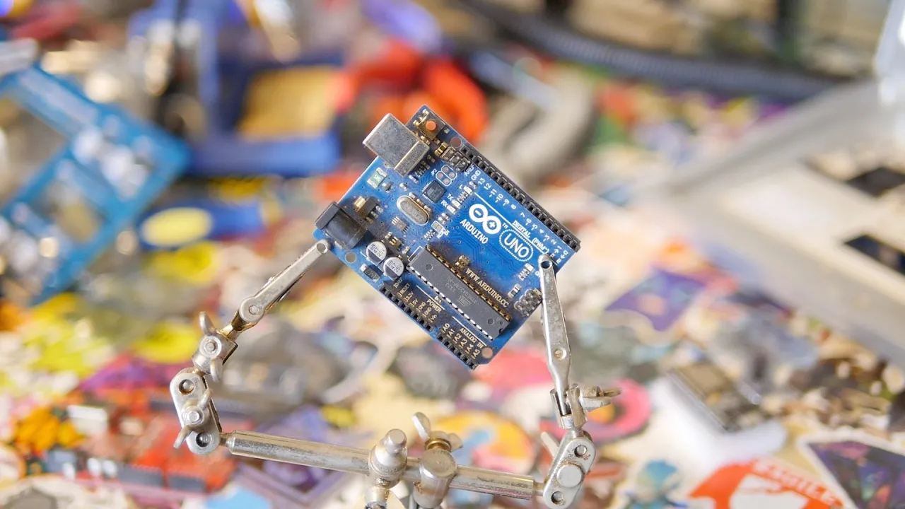
Arduino is a simple, low-cost board that enables users to work with microcontrollers. The microcontroller serves as the brain, found in many devices. Arduino Uno contains: USB port, power jack, 5V regulator, reset button, and analog input pins (A0-A5). The ATmega328P microcontroller has 2KB SRAM, 32KB Flash memory, and 1KB EEPROM. Arduino is open source, allowing design modifications. The Arduino IDE provides a comprehensive interface for development: code editor with syntax highlighting, compile/upload buttons, Tools menu for board selection, Sketchbook for project organization, and Serial Monitor for debugging. Shortcuts like Ctrl+Z, Ctrl+U, and Ctrl+R streamline the development process. The IDE automatically detects connected boards and COM ports.
Click to watch →
What Is Arduino? What Can You Do With It? Explained
103.2K
The Arduino IDE provides a user-friendly interface for programming microcontrollers. Setup involves selecting the correct board type and COM port, with third-party boards requiring additional USB serial drivers. Arduino programming extends C language with simplified syntax. Every program requires two essential functions: setup() runs once for initialization, and loop() runs continuously for main logic. Functions use curly braces and require semicolons. pinMode() configures pin direction, digitalWrite() controls output states, and delay() manages timing. The built-in LED variable (LED_BUILTIN) ensures code portability across different Arduino models.
Click to watch →
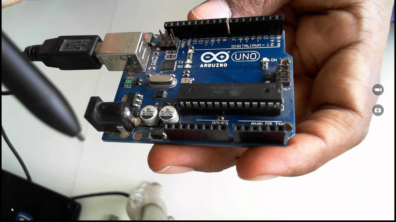
Beginning with Internet of Things IoT for Developers
171.5K
Arduino programming uses C-based sketches written in a simplified version of C. The Arduino IDE provides tools for writing, compiling, and uploading code to the board. The IDE includes a Serial Monitor for viewing output. Arduino programs have only two main constructs: setup() (runs once at startup) and loop() (runs continuously). Built-in functions include pinMode() for configuring pins as input or output, digitalWrite() for writing values to digital pins, and delay() for introducing time delays in milliseconds. Libraries are pre-written code that simplifies working with sensors and components, handling complex communication protocols and data interpretation.
Click to watch →

✅ El Programador que Te Ahorrará gastos en los Proyectos Electrónicos con ATtiny 85 o ATmega 328P PU
146K
This comprehensive section covers the foundational concepts of microcontroller programming using ATtiny 85, ATtiny 45, and ATmega 328P. The video explains how to build a programmer (quemador) that eliminates the need for external crystal oscillators and capacitors. Key topics include accessing the Arduino IDE for downloading programs and Gerber files for PCB manufacturing, understanding pin configurations for SPI programming (pins 13, 12, 11 for MISO, MOSI, SCK), and the role of the reset pin. The section details configuring the Arduino as an ISP programmer by downloading the ArduinoISP example, selecting the appropriate serial port, and verifying compilation. It also covers installing additional boards through the Board Manager, creating the necessary hardware folder structure, and copying board files. The video demonstrates burning the Arduino bootloader onto microcontrollers and programming them with internal 8 MHz oscillators.
Click to watch →
Deep Dive
Fundamentals of standard communication protocols, particularly I2C and SPI, used for sensor interfacing.
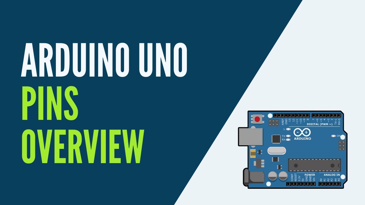
Arduino Uno - Pins Overview
104.3K
I2C (Inter-Integrated Circuit) and SPI (Serial Peripheral Interface) enable communication with external sensors and peripherals. I2C uses two wires: SDA (data) and SCL (clock), implemented on Uno via pins A4 and A5. Only one I2C module exists, so avoid using both SDA pins simultaneously. SPI offers faster data transfer than I2C but requires more wires: SCK (clock), MISO (receive), MOSI (transmit), and SS/CS (chip select) per device. On Uno, these correspond to pins 13, 12, 11, and 10 respectively. SPI is not recommended for long wire runs due to signal degradation. Both protocols require power and ground connections. Choose I2C for longer distances and SPI for higher speed applications within short ranges.
Click to watch →

9- Communication Protocols _ Hardware
141
Communication protocols are standardized rules enabling electronic devices to exchange data reliably. They serve as a common 'language' allowing microcontrollers, sensors, and interfaces to understand each other. Protocols ensure data is transferred accurately without errors, which is critical for correct system operation. Standardization is essential because multiple manufacturers produce chips with communication interfaces, making interoperability possible. Serial communication transfers data one bit at a time over a single wire, while parallel communication transfers multiple bits simultaneously over multiple wires. UART (Universal Asynchronous Receiver/Transmitter) enables asynchronous serial communication without requiring a shared clock signal, using two wires: TX and RX, plus ground. UART data frames consist of a start bit, 8 data bits (LSB first), optional parity bit, and stop bit. I2C (Inter-Integrated Circuit) is a synchronous serial communication protocol using two wires: SDA and SCL. It supports multiple masters and slaves, with each slave having a unique 7-bit address. I2C uses open-drain configuration with pull-up resistors. Speed modes include Standard Mode (100 kbps), Fast Mode (400 kbps), and Fast Mode Plus (1 Mbps). SPI (Serial Peripheral Interface) is a synchronous serial communication protocol using four wires: MOSI, MISO, SCK, and SS. SPI supports full-duplex communication with high-speed data transfer (up to 10 Mbps or more). SPI communication begins when the master selects a slave by pulling its SS line low, then generates clock pulses on the SCK line for data transfer.
Click to watch →

Serial Protocol Fundamentals
29.1K
Serial transmission sends data one bit at a time over a shared bus, offering advantages over parallel transmission including longer distances, higher throughput, and support for more nodes; three common low-speed serial protocols are UART (asynchronous, two-wire, uses start/stop bits and optional parity for framing data), I2C (synchronous, two-wire, master-slave architecture with address-based communication and acknowledgment bits), and SPI (synchronous, four-wire, full-duplex with separate chip select lines for addressing slaves); each protocol defines how bits are formatted into messages and the rules for exchanging data between devices.
Click to watch →
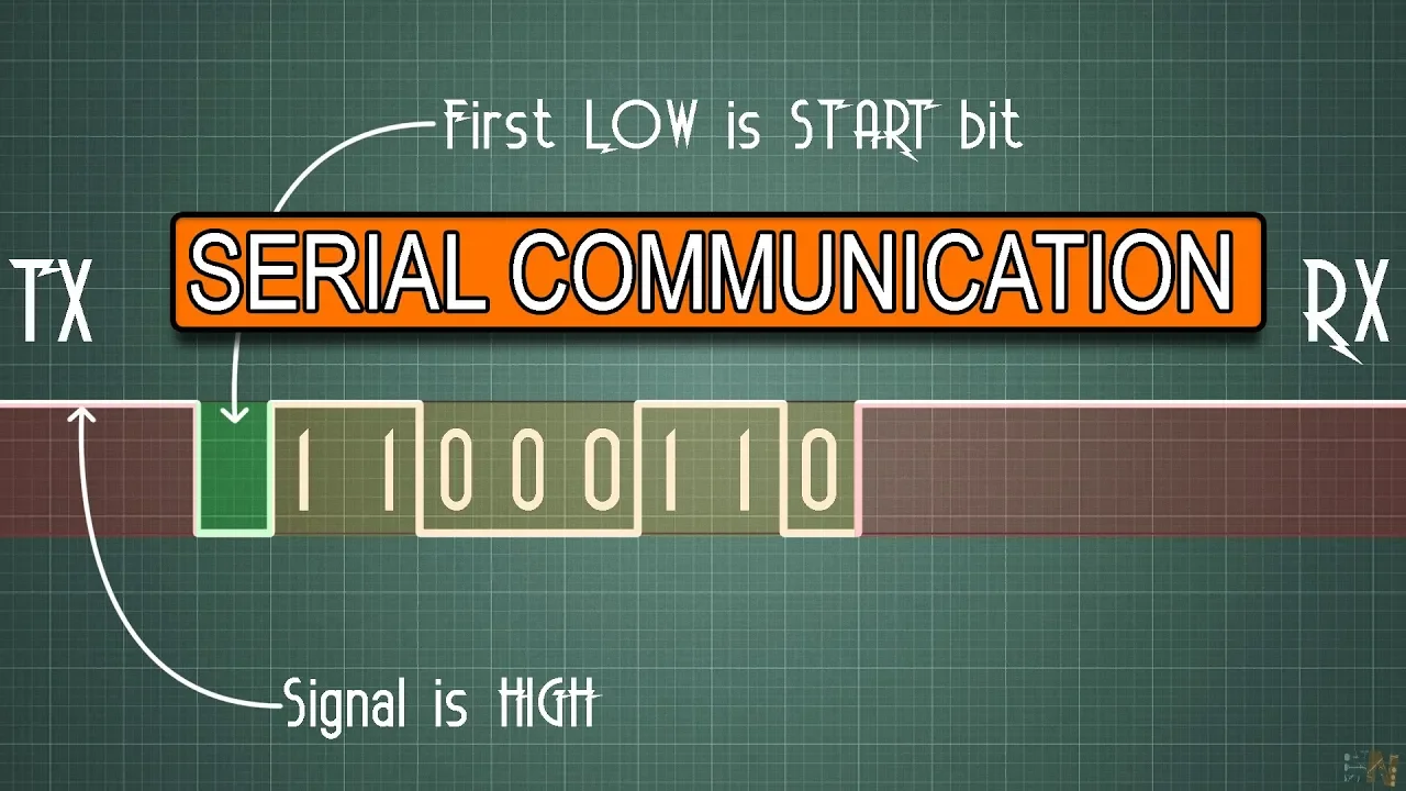
PROTOCOLS: UART - I2C - SPI - Serial communications #001
1.6M
This video explains three fundamental serial communication protocols used in microcontroller applications: UART (Universal Asynchronous Receiver Transmitter) uses two wires (TX/RX) with start/stop bits and a shared clock, requiring configuration of baud rate and data format; I2C (Inter-Integrated Circuit) uses two wires (SDA/SCL) with a clock line for synchronization and slave addressing, allowing multiple devices on one bus; SPI (Serial Peripheral Interface) uses four wires (MOSI/MISO/SCK/CS) for full-duplex communication without slave addressing, offering higher speed and lower power consumption but limited range. Each protocol balances trade-offs between connection count, speed, complexity, and range.
Click to watch →
Schematic Design - Landing Model Rockets Ep. 4
176.9K
I²C uses two lines (SDA for data, SCL for clock) to connect multiple devices on a shared bus, requiring unique device addresses. SPI uses four lines (MOSI, MISO, SCK, and CS) with a dedicated CS line per device, enabling faster communication but consuming more pins. Both protocols allow the processor to communicate with sensors (IMU, barometer) and storage devices (SD card, flash chip) efficiently.
Click to watch →
Deep Dive
Basic concepts of control theory, specifically the distinction between open-loop and closed-loop feedback systems.
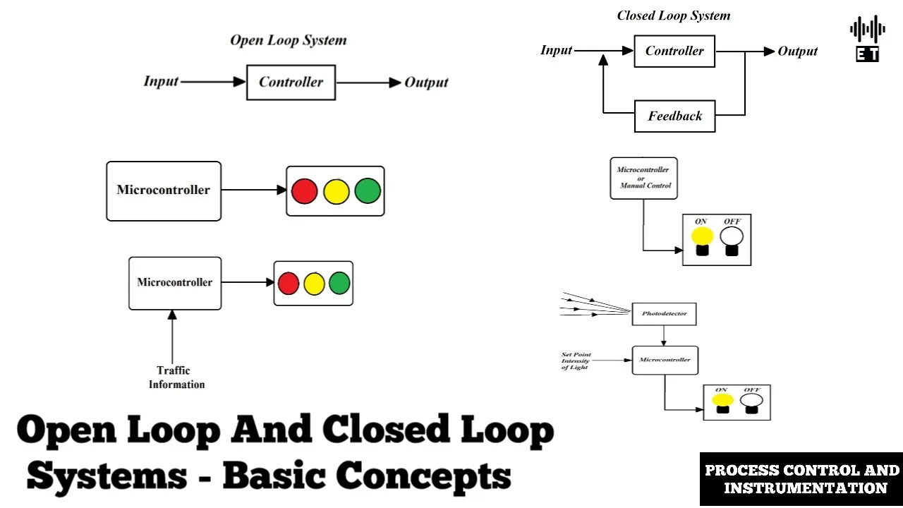
Open Loop And Closed Loop Systems | Basic Concepts | Process Control
4K
This section covers the core definitions and characteristics of open loop and closed loop systems. An open loop system operates without a feedback path from output to input, meaning the output is not measured or compared with a reference set point. Control action is independent of the desired output, making these systems simple in design, less costly, easier to install, and requiring minimal maintenance. In contrast, a closed loop system incorporates a feedback path with a controller that continuously monitors output using sensors, compares it against a set point, and adjusts the input based on the error signal to minimize the gap between actual and desired output. Closed loop systems offer better accuracy but require more complex circuitry, higher costs, and regular maintenance.
Click to watch →

Control systems | Open loop and Closed Loop | Introduction | Lec-01
13.3K
Control systems are classified into open loop and closed loop types. Open loop systems have input, controller, and process with no feedback path connecting output back to controller. Closed loop systems include a feedback path where output is measured by a measuring element and fed back to the controller. The controller compares input with feedback to generate an error signal, which modifies the input to achieve desired output. This automatic adjustment distinguishes closed loop systems from open loop ones.
Click to watch →

L01 Revision of Control System | Basic Concept | GATE 2026 #umeshdhande
5.2K
A control system is a system with a controller that produces a controlled output, where the key distinction between open loop and closed loop systems lies in feedback: open loop systems have a controlling mechanism independent of the output (no feedback), while closed loop systems have a feedback mechanism that depends on the output. The closed loop transfer function for a negative feedback system is given by G(s)/(1 + G(s)H(s)), where G(s) is the forward path gain and H(s) is the feedback path gain. This feedback structure makes closed loop systems less sensitive to parameter variations in the forward path, which is why they are preferred for reliable control applications.
Click to watch →
CONTROL SYSTEM - 1 OPEN LOOP & CLOSED LOOP SYSTEM - TAMIL
61.1K
Open-loop systems apply input without feedback, while closed-loop systems use feedback to compare actual output with desired output. Open-loop systems have a simple input-to-output structure with no feedback path. Closed-loop systems include a feedback mechanism that continuously monitors output and adjusts control actions to minimize error. The key difference is that closed-loop systems can compensate for disturbances and maintain desired output despite external variations, making them more suitable for applications requiring precise control.
Click to watch →
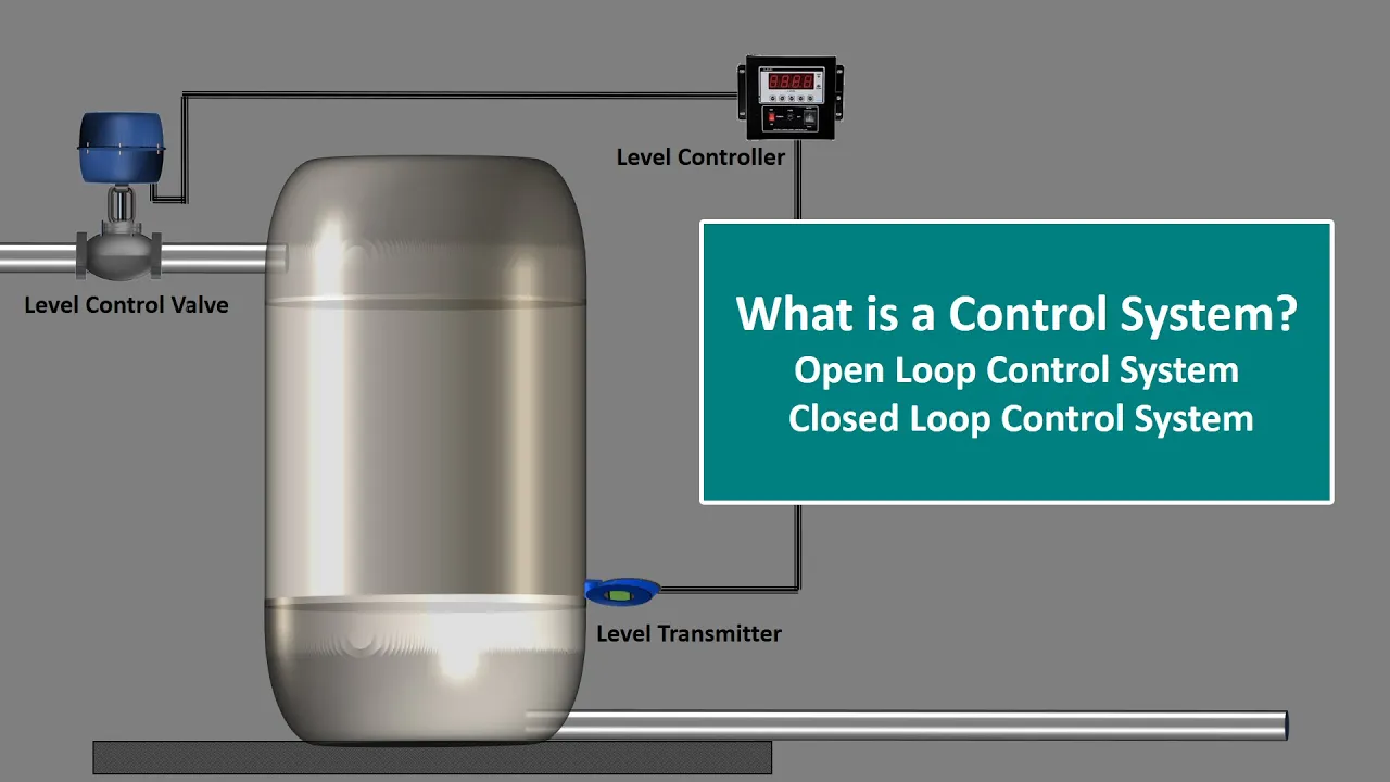
What is Control System.Control System Engineering.Open Loop and Closed Loop Control System.Explained
48.1K
A control system is an arrangement of components that performs a specific task by transforming input through a process to produce output; it can be classified into open loop systems (which operate without feedback and assume output meets requirements) or closed loop systems (which use feedback to automatically adjust and maintain desired output).
Click to watch →
Deep Dive
Electrical fundamentals including voltage division, current sensing techniques, and safe power supply handling.

Ninguém te Explicou ATÉ HOJE! Aprenda AGORA Para Entender a Placa! Eletronica Facil
912
Resistors are fundamental components in switched power supplies, serving multiple critical functions. Voltage division circuits monitor AC input voltage through series resistor networks for brown-out protection (BNO pin), preventing IC damage when voltage falls below safe thresholds. High-value resistor networks (1.5MΩ+) supply the VCC pin, limiting current to microampere levels while charging the VCC capacitor. Current sense resistors (shunt resistors, typically <1Ω) monitor circuit current by creating proportional voltage drops (V = I × R) for overload protection. Component designation systems use standardized codes: 'R' for resistors, 'U' for primary circuit ICs, and 'S' for secondary circuits. Understanding these resistor applications is essential for power supply design and troubleshooting.
Click to watch →

Một bài học về mạch bảo vệ trên điều hòa Inverter, đây là kiến thức chuyên sâu giúp bạn sửa pan khó.
1.4K
The overcurrent protection circuit uses a voltage divider (221 ohm and 3.74K ohm resistors) to create a 0.3V reference voltage from a 5V source. The current sensing resistor (0.02 ohm) converts current to voltage using Ohm's Law (V = I × R). For 15A maximum current, this produces exactly 0.3V. The comparator compares this voltage against the reference. When current exceeds 15A, the input voltage exceeds the reference, causing the output to generate a 5V pulse that interrupts the power IC.
Click to watch →

Amateurfunkvorlesung Klasse E -- Lektion 5. Internationaler Funkbetrieb und Lektion 6. (Teil 1)
2.8K
This section covers voltage, current relationships, and electrical safety fundamentals. Voltage represents potential difference between points in an electric field, calculated as the integral of electric field along a path, measured in volts (named after Volta). Reference points establish voltage measurements: a 9-volt battery with 0V reference shows potentials of 0V, 3V, 6V, and 9V at different points. Electric current I = dQ/dt represents charge flow rate, with Q = I×t for constant current. One ampere equals one coulomb per second. Electrical safety depends critically on voltage type and current path: DC becomes dangerous above 120V, AC above 50V at 50Hz. With typical body resistance of 1kΩ, 120V DC produces ~120mA, sufficient to cause ventricular fibrillation. Always assume stored energy in capacitors even when equipment appears powered off.
Click to watch →
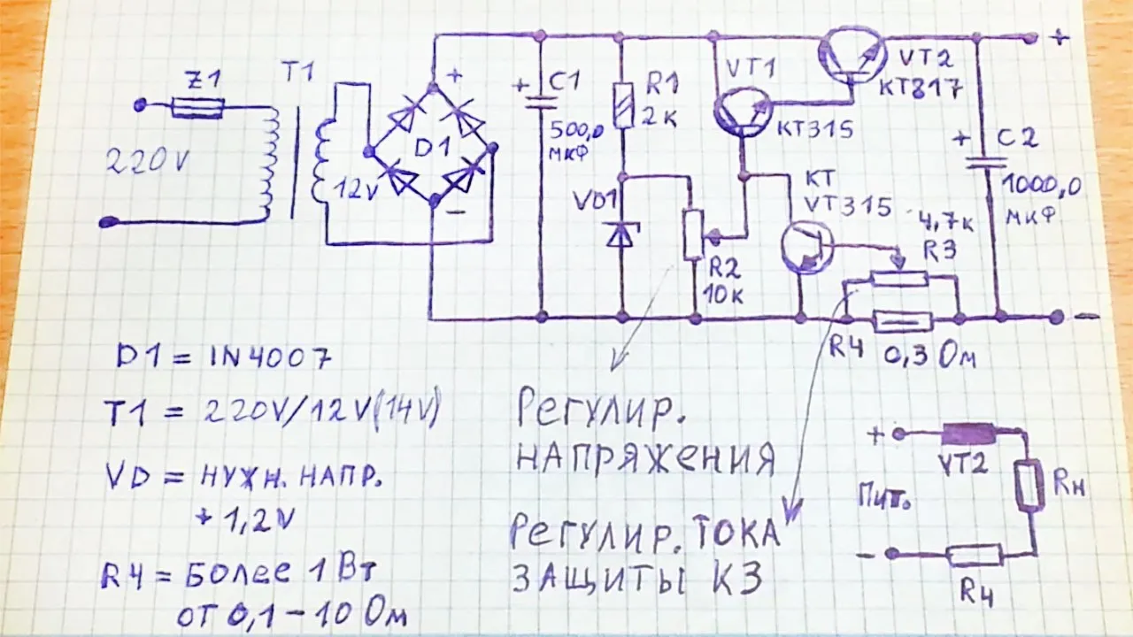
Простая схема регулируемого блока питания на транзисторах с защитой от перегрузки по току и КЗ
277.3K
In a power supply circuit, current sensing can be achieved by placing a small sense resistor in series with the load. When current flows through this resistor, a voltage drop develops across it proportional to the current. This voltage is divided among multiple resistors in the circuit according to their resistance values—higher resistance results in higher voltage drop. By monitoring this divided voltage, the circuit can detect changes in load current.
Click to watch →

Samsung over current error repaired by Student Shridhar 1
2.2K
The current sensing circuit uses a comparator IC with voltage dividers to measure current. The voltage divider is created using a 4.4V reference (pin 5) and a voltage divider network. The expected voltage at the divider output should be approximately 370mV, but in this case, it was reading 307.5mV, indicating a fault in the voltage divider circuit.
Click to watch →
Prerequisite Knowledge
- Concept 01Basic principles of Brushless DC (BLDC) motor operation and the core concept of Field Oriented Control (FOC).
- Concept 02Proficiency with the Arduino IDE, basic microcontroller programming, and interfacing with hardware pins.
- Concept 03Fundamentals of standard communication protocols, particularly I2C and SPI, used for sensor interfacing.
- Concept 04Basic concepts of control theory, specifically the distinction between open-loop and closed-loop feedback systems.
- Concept 05Electrical fundamentals including voltage division, current sensing techniques, and safe power supply handling.
Subsequent Learning
- Step 01Advanced PID controller tuning for precise torque, velocity, and position control of BLDC motors.
- Step 02Implementation of space vector pulse width modulation (SVPWM) and direct-quadrature (d-q) current control.
- Step 03Integration of high-resolution magnetic or optical encoders to achieve optimal closed-loop performance.
- Step 04Designing real-world robotic applications such as haptic controllers, self-balancing robots, or robotic arm joints using FOC.
- Step 05Thermal management and efficiency optimization strategies for motor driver circuits under continuous loads.
Setup & Wiring
Interface Tests
Position Control
Speed & Current
Setup & Wiring
0:11Playing Section
- 1
Stack SimpleFOX shield on Arduino Uno and connect via USB.
- 2
Connect motor phases and encoder via analog and I2C interfaces.
- 3
Verify connections with provided circuit diagrams.
Limitations of Low-Cost Microcontrollers and Maker-Grade Hardware for Field-Oriented Control
While the Makerbase SimpleFOC shield and Arduino ecosystem offer an accessible, low-cost entry point for learning Field-Oriented Control (FOC), professional and industrial applications typically reject this setup due to significant performance and reliability bottlenecks. Standard 8-bit or low-end 32-bit Arduinos lack the computational power required for high-frequency current loop calculations (typically needing 10–20 kHz), leading to control latency, torque ripple, and acoustic noise. Furthermore, maker-grade drivers like Makerbase often suffer from poor thermal dissipation and noisy analog current-sensing circuitry. For robust, high-performance, or safety-critical applications, engineers favor dedicated motor-control platforms (such as ODrive, VESC, or Texas Instruments InstaSPIN) utilizing advanced Digital Signal Processors (DSPs) or ARM Cortex-M4/M7 microcontrollers with hardware-accelerated math and superior noise-isolated PCB layouts.
Deep Dive
Advanced PID controller tuning for precise torque, velocity, and position control of BLDC motors.

My Engineering Thesis is Imploding
10K
Motor controllers use cascade PID structure: current loop (innermost), velocity loop (middle), and position loop (outermost). Position commands translate to velocity, then current, processed by Field Oriented Control (FOC) for efficient torque generation. Each controller has P, I, D parameters requiring tuning. Velocity tuning: increase gain until motor turns poorly, then reduce by 50%. Position tuning: find critical oscillation point and slightly reduce gain. Velocity integrator gain is typically 10× velocity gain. The most common technique is systematic guess and check.
Click to watch →

MD80 x CANdle - motion modes
1.4K
Velocity PID mode uses a single PID controller with proportional, integral, derivative gains, integral windup limit, and max torque parameter. Max torque limits maximum output torque regardless of PID calculations, serving as a critical safety feature. Position PID mode employs cascaded architecture: a position controller outputs target velocity based on desired position, while a velocity controller outputs motor torque to maintain that velocity. This enables advanced motion control with predefined maximum velocity and torque limits. Always tune velocity controller first before position controller. Max velocity limits shaft velocity between position points, while max torque limits applied force. High values produce aggressive, strong-holding behavior; low values create slow, easily disturbed movement. These parameters enable safe, controlled motion profiles tailored to specific application requirements.
Click to watch →

PID Control of a Brushless DC Motor
19.8K
This video demonstrates how to automatically tune the gains of a cascaded PID controller for a brushless DC motor with trapezoidal back-EMF using the Closed-Loop PID Autotuner block in Simulink Control Design. The method involves sequentially tuning the inner voltage loop and outer speed loop by injecting excitation signals during closed-loop operation to estimate plant frequency response, then computing optimal PID gains that achieve a target phase margin of 60 degrees and specified bandwidths (400 rad/sec for voltage loop, 100 rad/sec for speed loop), resulting in improved reference tracking performance compared to initial controller settings.
Click to watch →

Position Controlling of a Brushless Motor with an Incremental Encoder using SOLO
7K
Motor control requires sequential tuning of torque, speed, and position controllers. Torque controller tests verify constant torque output under load. Speed controller tuning adjusts kp and ki gains for desired dynamic response—kp affects response speed, ki eliminates steady-state error. Position controller tuning follows with higher gains than speed controller. Iterative gain adjustment balances response speed against stability. Speed limit parameters define maximum traversal velocity. Properly tuned controllers enable precise position tracking with minimal overshoot and settling time. The process requires systematic testing and parameter refinement to achieve optimal performance.
Click to watch →

InstaSPIN-BLDC with the DRV-8312 and 28035 Piccolo
18.7K
This section covers PI control loop implementation and advanced motor control strategies. Velocity control mode implements closed-loop speed regulation by comparing commanded rotor speed with actual speed (estimated from commutation times) to generate an error signal through proportional and integral gain paths. The P-term sets system stiffness and speed tracking accuracy. The I-term eliminates steady-state error by integrating the error signal. Tuning starts with low gains to avoid oscillation, then increases for desired performance. Current control mode regulates torque by comparing commanded current with actual bus current through a PI control loop. Cascade mode combines velocity and current control loops, with the velocity loop output feeding into the current loop and being clamped by a maximum current limit. This provides comprehensive motor control by managing both speed and torque requirements simultaneously.
Click to watch →
Deep Dive
Implementation of space vector pulse width modulation (SVPWM) and direct-quadrature (d-q) current control.

SVPWM - discrete implementation
27K
Space Vector PWM (SVPWM) is a modulation technique for three-phase inverters where three-phase reference voltages are converted to time durations using the relationship ta = ts × va/vdc, tb = ts × vb/vdc, and tc = ts × vc/vdc, with ts being the carrier period and vdc the DC bus voltage; the algorithm calculates tmax, tmin, and teff (effective time within the envelope), then applies an offset to handle negative time values, and finally loads these values into compare registers of a microcontroller/DSP to generate PWM signals, with dead time included between complementary switches to prevent shoot-through.
Click to watch →

Space Vector PWM
9.2K
Space Vector PWM (SVPWM) is an advanced modulation technique for voltage source inverters that achieves full DC bus utilization without additional switches. The inverter topology consists of three legs with complementary IGBT switches per leg, following rules: one switch ON per leg, no simultaneous ON of both switches, and small dead time between transitions. Phase voltages relate to pole voltages through common mode voltage V_on = (V_a0 + V_b0 + V_c0)/3. Sine triangle PWM limits peak phase voltages to V_DC/2. SVPWM defines space vectors by multiplying phase voltages by orientation factors (0°, 120°, 240°) and summing: V_s = V_a × e^(j0) + V_b × e^(j2π/3) + V_c × e^(-j2π/3). The inverter has 8 switching states: 2 zero states and 6 active states at 60-degree intervals. Space vector synthesis uses adjacent active vectors and zero vectors with duty ratios: D_V1 = (M_V × sin(α - 30°))/sin(60°), D_V2 = (M_V × sin(α + 30°))/sin(60°). The maximum space vector amplitude is (√3/2) × V_DC, corresponding to maximum phase voltage of (2/3)V_DC and RMS line-to-line voltage of 0.707 × V_DC, representing a 20% improvement over sine triangle PWM. SVPWM is implemented using carrier modulation with common mode voltage offset, following a symmetric switching pattern. It is essential for vector control, direct torque control, and V/f control applications in motor drives and grid-connected inverters.
Click to watch →

TMS320F28379D, LAUNCHXL-F28379D - Implementation of other PWMs for 3ph : SVPWM, DPWM1 and DPWM2
2K
The complete SVPWM algorithm involves: (1) Tracking the reference vector angle θ across the 0-2π range at grid frequency angular velocity, (2) Identifying the current sector based on θ, (3) Calculating duty cycles for the two adjacent space vectors using trigonometric functions, (4) Applying the computed duty cycles to generate PWM signals for the three phases. Simulation results demonstrate that SVPWM produces sinusoidal output voltages with characteristic waveforms. The technique maintains the same volt-second area as SPWM while achieving higher DC bus utilization and reduced switching losses.
Click to watch →
![SVPWM : Explication mli vectorielle avec simulation MATLAB/Simulink [CC English]](https://i.ytimg.com/vi_webp/FOQvHQX4QHY/maxresdefault.webp)
SVPWM : Explication mli vectorielle avec simulation MATLAB/Simulink [CC English]
37K
The SVPWM implementation in MATLAB/Simulink uses an S-function with standard template structure, featuring 4 inputs and 10 outputs. Key variables are declared as doubles except for the integer sector number. The Clarke transformation converts three-phase references to alpha-beta components. Sector determination uses arctangent functions with rounding to identify the 60-degree sector. Each sector requires specific commutation logic with unique threshold values. Commutation times are divided by two for symmetry. The algorithm compares the reference angle modulo against thresholds to determine switching states, producing complementary duty cycles that ensure proper inverter operation.
Click to watch →

Implementing Digital Motor Control
57.7K
Space vector PWM uses six key sector vectors representing switch states (e.g., 100, 011). The desired voltage vector is projected onto adjacent sector vectors, and duty cycles are calculated and updated continuously (at 10-20 kHz). This creates a waveform that appears as a sine wave after low-pass filtering. The technique injects third harmonic by tapering the peak, which doesn't affect Y-connected or delta-connected motors. Benefits include reduced DC bus voltage requirements, lower switching losses, reduced EMI, and more efficient motor control.
Click to watch →
Deep Dive
Integration of high-resolution magnetic or optical encoders to achieve optimal closed-loop performance.
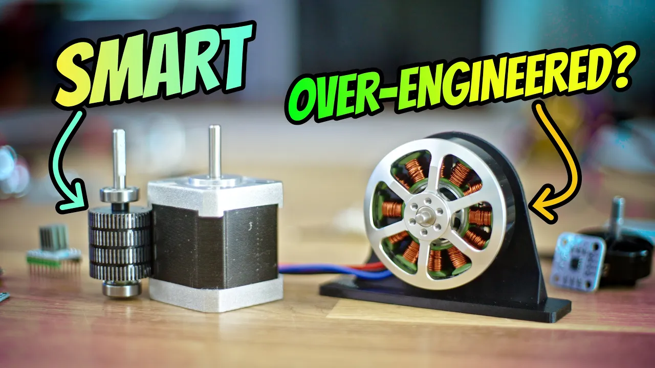
Steppers vs Servos in 3D Printers: An Engineering Analysis
280.8K
Positional feedback transforms any motor into a servo through encoders—magnetic or optical devices measuring rotational position. Magnetic encoders attach a magnet to the shaft and use chips to measure position, while optical encoders use graded transparent films or rotating sensors. Closed-loop systems detect external disturbances and compensate, unlike open-loop systems that lose steps silently. FOC requires precise rotor position knowledge to optimally control each coil, stopping current entirely when at target position. This contrasts with constant stepper energization, enabling dynamic current adjustment based on actual torque needs rather than fixed patterns.
Click to watch →
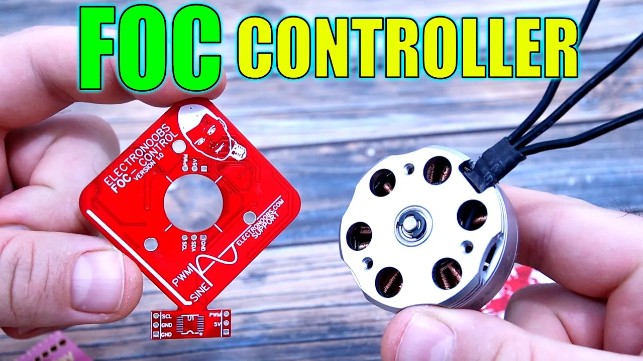
FOC Driver Controller PCB - Slow Brushless Control
140.5K
Open loop FOC has a critical limitation: external forces can cause position drift without the system detecting or correcting it. Closed loop control addresses this by integrating magnetic encoders that provide continuous position feedback. Radial magnets are essential because they create two-polarity magnetic fields that interact properly with encoders, unlike standard axial magnets. The encoder outputs a PWM signal where pulse width corresponds to the detected rotation angle. This feedback enables the system to actively track and correct position errors. Without proper encoder integration, the system fails to maintain accurate positioning under load. The complete FOC implementation demonstrates how combining sinusoidal signal generation, motor driving, and position sensing creates a powerful control system suitable for precision robotics applications.
Click to watch →
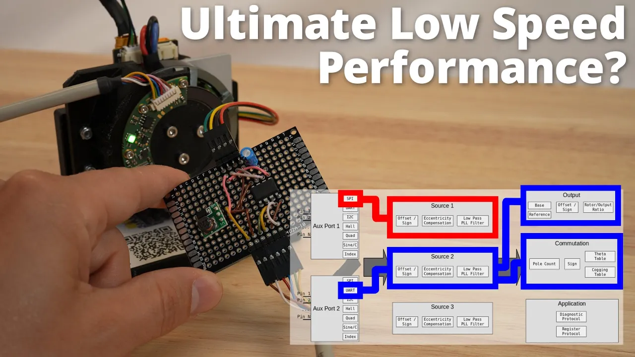
9.5 encoder strategies for open source bldc control
14.2K
This concluding section covers specialized high-resolution encoder interfaces and open-loop control alternatives. The RLS AxiM-2 uses magnetic ring technology with RS-422 UART interface, requiring voltage boosting and transceivers, while the iC-Haus iC-PZ employs reflective optical sensing with SPI interface offering 24-bit resolution. Both demonstrate how higher-resolution encoders significantly improve low-speed performance and stiffness compared to standard encoders. The section then introduces fixed voltage mode for open-loop motor control, driving motors like stepper motors without encoders by applying constant phase voltage. This provides open-loop velocity and position control but lacks closed-loop accuracy and can skip steps under load. Finally, general-purpose I/O capabilities are demonstrated, allowing any pins to function as digital inputs/outputs or analog inputs when not used for encoder functions, with values accessible via diagnostic tools or register protocols.
Click to watch →

How different Encoder systems influence the control loop (Detailed procedure for each encoder)
226
Different encoder systems significantly impact motion control loop performance; optical encoders offer the highest precision with minimal noise, enabling higher loop gains and better disturbance compensation, while magnetic incremental and absolute encoders provide good performance with some noise, and linear Hall sensors show more oscillations in speed response. The choice of encoder affects both speed and position loop stability and responsiveness.
Click to watch →

Why the brushless controllers are awesome for robotics
145.2K
Closed-loop position control compares actual rotor position (from encoder) against a setpoint to compute error. Maximum torque requires 90-degree phase advance relative to rotor position, implemented as +12 or -12 steps in the 48-value array. SPI-based encoder reading eliminates PWM noise, providing stable position tracking. The control algorithm maps encoder values to electronic shaft positions, applies proportional torque based on error magnitude, and includes experimental offset compensation for mechanical misalignment. This enables precise motor positioning with minimal vibration.
Click to watch →
Deep Dive
Designing real-world robotic applications such as haptic controllers, self-balancing robots, or robotic arm joints using FOC.

Counterbalancing a Robot's Arm Using Springs WVROX 2020
14.6K
Team applications demonstrate practical counterbalancing: 2014 intake used spring balancing to reduce pneumatic size, 2018 climber used pulley-routed springs for long-arm balancing. Verification shows properly counterbalanced arms remain stationary at any position, gliding equally in both directions due to friction. Mathematical design philosophy enables precise upfront calculations rather than iterative trial-and-error with gearboxes.
Click to watch →
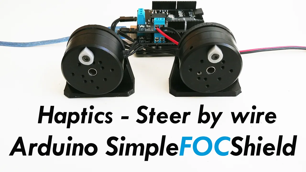
Arduino Field Oriented Control (FOC) Haptic control example - SimpleFOCShield
94.7K
Haptic control creates virtual links between motors to enable force feedback, where users can feel forces from one motor when interacting with another; this is achieved through software algorithms that synchronize motor positions or couple position with velocity, allowing applications like interactive gauges or throttle controls where users can both command and sense motor behavior in real-time.
Click to watch →
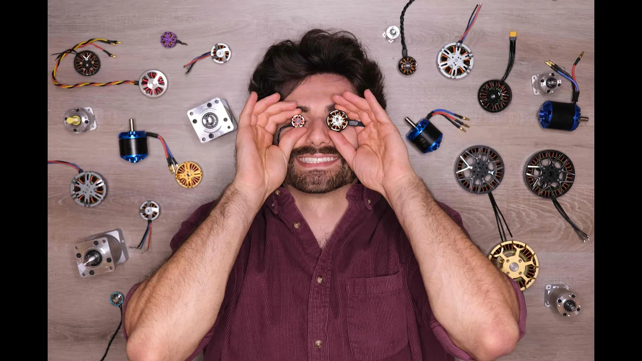
DIY Robot Arm Details - Ep. 2
2.7K
Field Oriented Control (FOC) is the process by which motor controllers rapidly sequence power to electromagnetic coils in the motor to push and pull magnets with the right force at the right time. The controller also reads rotor angle and measures current through motor windings to calculate torque. FOC operates at high speeds, about 30,000 times per second, for precise motor control.
Click to watch →
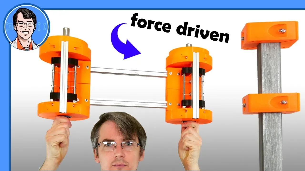
Building a Force Driven Robot Arm #1 | James Bruton
60.2K
A force-controlled robot joint uses springs between the servo and finger mechanism to create compliance. As more force is applied, the spring stretches proportionally. By measuring the finger position with a flex sensor and knowing the servo position, the system can calculate the applied force. This allows the robot to actively back-drive joints by setting desired force levels rather than fixed positions, making the joint compliant and safe for interaction with humans or delicate objects.
Click to watch →

I Built a Robot Dog Using... Rope?
850K
Field-Oriented Control (FOC) is an advanced motor control technique that transforms ordinary brushless motors into high-precision actuators capable of position, velocity, and torque control. FOC controllers enable smooth, responsive motor operation by precisely managing the magnetic fields within the motor, allowing for sophisticated robotic movements and dynamic behavior.
Click to watch →
Deep Dive
Thermal management and efficiency optimization strategies for motor driver circuits under continuous loads.
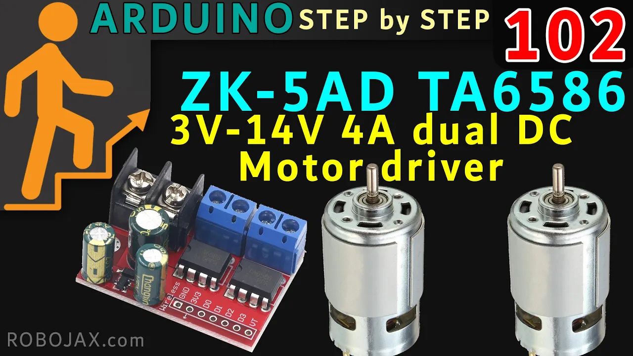
Lesson 102: Using ZK-5AD 4A Dual DC Motor Driver TA6586 4A 14V The best Motor Driver - RJT428
17.8K
This section demonstrates thermal management for motor drivers. Without heatsink, the TA6586 can handle 4A continuously at room temperature (reaching 59°C after 10+ minutes). At 5A, thermal shutdown activates automatically. Adding a heatsink allows the chip to handle higher currents (5-7A) by improving heat dissipation. The demonstration shows thermal imaging of the chip at different current levels, with temperatures rising from 59°C at 4A to 77°C at 5A. The recommended continuous current is 5A with proper heat dissipation, with maximum capability of 7A.
Click to watch →
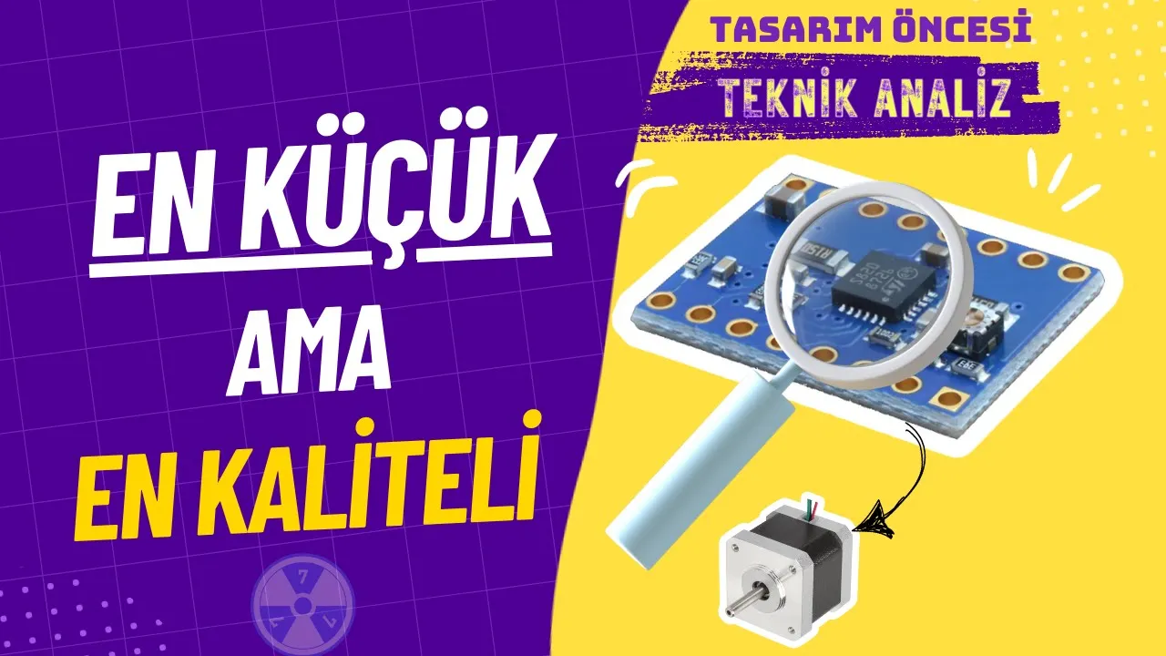
Datasheet İncelemek Bu Kadar KOLAY! | A4988 Kullanmayın! / JLCPCB
31K
This segment covers thermal management design with heatsinks and thermal vias. The presenter explains how thermal vias reduce junction-to-bottom resistance to ~1°C/W. With heatsinks on both top and bottom, the total thermal resistance becomes ~9.32°C/W (parallel paths). The calculation shows maximum power dissipation of 8.58W with Tj_max = 120°C and Ta = 40°C. The segment demonstrates calculating maximum motor current from thermal limits: with 8.58W power limit and 5V motor, maximum current is 1.716A RMS (3.432A peak). Motor driver enable control and fault protection mechanisms are explained, including enable/disable pins and disable timing calculation using R × C × ln(Vcc/(Vcc - Vref)). PWM timing parameters (rise time, fall time, off time) are explained, with rise/fall times of 20ns and off time of 13μs enabling ~77kHz maximum PWM frequency. The segment provides comprehensive motor driver selection criteria based on current rating, microstepping resolution, PWM timing capabilities, thermal management, and cost.
Click to watch →

Укрощение молнии: Как мы создавали драйвер на 3000 В за наносекунды.
5.3K
Thermal imaging identifies hot spots revealing power dissipation patterns in driver circuits. Component heating affects reliability and performance. Real electro-optic crystal loads (with higher capacitance than unloaded conditions) can actually improve pulse characteristics. The driver must be designed for actual load conditions, which may differ significantly from unloaded measurements.
Click to watch →

Electrical Drive | Utilization of Electrical Energy | Lec 12 | SSC JE, RRB JE Exam | Rahul Sharma
45.8K
Load-speed relationships vary by application: constant load (conveyors), proportional load (fans, blowers), and inverse load (grinding machines). Duty cycles determine motor thermal design: continuous duty allows steady-state temperature, short duty prevents reaching steady-state, and intermediate duty varies. Intermittent duty with starting and breaking (drilling machines) requires considering heat from both starting and braking periods. Active loads work against drive motion (gravity in elevators) while passive loads work in the same direction (friction in bearings). Proper classification ensures motor thermal management and longevity.
Click to watch →

Webinar: How to Estimate Motor Driver Power Dissipation
1.3K
This section covers the foundational concepts of thermal management in motor driver IC design. Key topics include: (1) Motor load current mission profiles with three distinct phases—T1 (inrush current at startup), T2 (steady-state operation), and T3 (stall condition)—and their impact on thermal behavior; (2) Thermal resistance definition as temperature difference divided by heat flow, measured in Kelvin/Watt or °C/Watt; (3) Thermal capacitance representing heat energy storage capacity, dependent on material properties and geometry; (4) Transient heat flow dynamics where the die heats first, followed by lead frame and PCB, before reaching steady-state; (5) The importance of estimating junction temperature evolution throughout the mission profile for safety and reliability. These fundamentals establish why accurate thermal analysis is critical for motor driver design.
Click to watch →
Setup & Wiring
Interface Tests
Position Control
Speed & Current
Setup & Wiring
0:11- 1
Stack SimpleFOX shield on Arduino Uno and connect via USB.
- 2
Connect motor phases and encoder via analog and I2C interfaces.
- 3
Verify connections with provided circuit diagrams.
Limitations of Low-Cost Microcontrollers and Maker-Grade Hardware for Field-Oriented Control
While the Makerbase SimpleFOC shield and Arduino ecosystem offer an accessible, low-cost entry point for learning Field-Oriented Control (FOC), professional and industrial applications typically reject this setup due to significant performance and reliability bottlenecks. Standard 8-bit or low-end 32-bit Arduinos lack the computational power required for high-frequency current loop calculations (typically needing 10–20 kHz), leading to control latency, torque ripple, and acoustic noise. Furthermore, maker-grade drivers like Makerbase often suffer from poor thermal dissipation and noisy analog current-sensing circuitry. For robust, high-performance, or safety-critical applications, engineers favor dedicated motor-control platforms (such as ODrive, VESC, or Texas Instruments InstaSPIN) utilizing advanced Digital Signal Processors (DSPs) or ARM Cortex-M4/M7 microcontrollers with hardware-accelerated math and superior noise-isolated PCB layouts.
Basic principles of Brushless DC (BLDC) motor operation and the core concept of Field Oriented Control (FOC).
Proficiency with the Arduino IDE, basic microcontroller programming, and interfacing with hardware pins.
Fundamentals of standard communication protocols, particularly I2C and SPI, used for sensor interfacing.
Basic concepts of control theory, specifically the distinction between open-loop and closed-loop feedback systems.
Electrical fundamentals including voltage division, current sensing techniques, and safe power supply handling.
Advanced PID controller tuning for precise torque, velocity, and position control of BLDC motors.
Implementation of space vector pulse width modulation (SVPWM) and direct-quadrature (d-q) current control.
Integration of high-resolution magnetic or optical encoders to achieve optimal closed-loop performance.
Designing real-world robotic applications such as haptic controllers, self-balancing robots, or robotic arm joints using FOC.
Thermal management and efficiency optimization strategies for motor driver circuits under continuous loads.
3.7K views38likes8:10@makerbaseteam4217Original Release: 2021-04-07
this lesson introduces the basic tests of simple [ __ ] first we stack the corresponding ports of the simple foxshield motherboard and the arduino uno motherboard then we connect the arduino uno board to the pc with a usb cable next we connect the three phase wires of the motor to the interface of the simple fox shield main board since the encoder of the motor has two interfaces we will introduce the connection methods respectively below we connect the analog interface to the simple fox motherboard through the is5600 a cable this is the connection diagram of the motor connected to the motherboard through the analog interface we connect the i2c interface to the simple fox shield main board via a dupont cable this is the connection diagram of the motor connected to the motherboard through the i2c interface first we open the analog interface test program magnetic sensor analog example in the simple foc library example next we configure the development board and port first select the development board arduino uno and then select the port after the configuration is complete we click upload to burn the motherboard now the program has been burned next we open the serial monitor the serial monitor continuously returns the position and speed of the motor toggle the motor you can observe the motor position and speed change now the analog interface test has been completed first we open the i2c interface test program magnetic sensor by 2c example in the simple foc library example we click upload to burn the motherboard now the program has been burned next we open the serial monitor the serial monitor continuously returns the position and speed of the motor toggle the motor you can observe the motor position and speed change now the i2c interface test has been completed first we open the closed loop position test program velocity control in the simple foc library example shield the 13th line of code unlock the 15th line of code modify the 20th line of code modify the 41st line of code modify the 57th line of code modify the 60th line of code after the program is modified we click upload to burn the motherboard now the program has been burnt toggle the motor and after releasing the motor the motor returns to the initial position indicating that the motor has entered the closed loop mode next we open the serial monitor after it show motor ready we can send command to control the motor send t6.8 the motor will run to the position 6.8 send t0 the motor will run to the position 0.
now the closed loop position test has been completed first we open the closed loop speed test program angle control in the simple foc library example shield the 16th line of code unblock the 18th line of code modify the 22nd line of code modify the 43rd line of code modify the 56th line of code modify the 59th line of code after the program is modified we click upload to burn the motherboard now the program has been burned next we open the serial monitor after it show motor ready we can send command to control the motor send t2 the motor rotation send t6 the motor rotation send t0 the motor stops rotating now the closed loop speed test has been completed software can be downloaded from the makerbus mks github first we open the current sensing test code next we click upload to burn the motherboard now the program has been burned next we open the serial monitor the serial monitor continuously returns the current of phase a phase b and current amplitude of the motor toggle the motor you can observe the changes of phase a current phase b current and current amplitude after stopping toggling the motor the motor returns to the initial position now the current sensing test is complete this is all of the lesson thank you for watching
Up Next

26:56
RISC-V MangoPi MQ Pro, ESP32 Audio Board, DIY Haptics Review
@Electromakerio
15K views•2022-04-13

12:54
Triumph of Orthodoxy Icon: Byzantine Art & History Explained
@BenCallan
2.1K views•2024-08-06

9:49
FastAPI vs Flask vs Django: Choosing the Right Python Web Framework
@TechWithTim
302.5K views•2024-05-26

1:42
Game of Thrones Opening Credits: A Cinematic Analysis
@gameofthrones
46.3M views•2011-04-18
Related Study Plans & Knowledge Roadmaps
Structured learning paths in General & Interdisciplinary Studies
general-studies
Elevator Engineering: History, Physics & Cities
01From Hoists to Safety Brakes: The Dawn of Vertical Lift
02Hydraulic vs. Traction: The Engineering Physics of Elevators
03Modern Speed, Safety, and Algorithms
+ 2 more learning modules
12h5 modules
Explore Roadmap
general-studies
Rubber: Material Science, History & Geopolitics
01Origins of Natural Rubber & Mesoamerican History
02The Chemistry of Natural Rubber & Vulcanization
03The Geopolitics of the Rubber Boom & Colonization
+ 2 more learning modules
12h5 modules
Explore Roadmap
general-studies
Containerization: Evolution, Logistics & Trade
01Ancient Trade & Bulk Cargo: Amphorae to Barrels
02The Industrial Revolution & Cardboard Packaging
03The Containerization Revolution: Malcom McLean
+ 2 more learning modules
12h5 modules
Explore Roadmap
general-studies
Textile Tech: Evolution, Labor & Global Impact
01Pre-Industrial Textiles: Handloom & Cottage Industry
02Mechanization: The Spinning Jenny to the Power Loom
03The Factory System & Global Labor Transformation
+ 2 more learning modules
10h5 modules
Explore Roadmap