Inverse Kinematics of 2 and 3 DOF Robots Explained

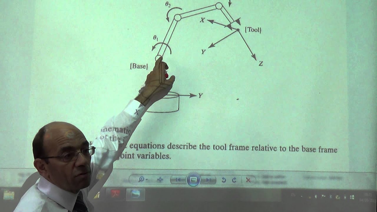
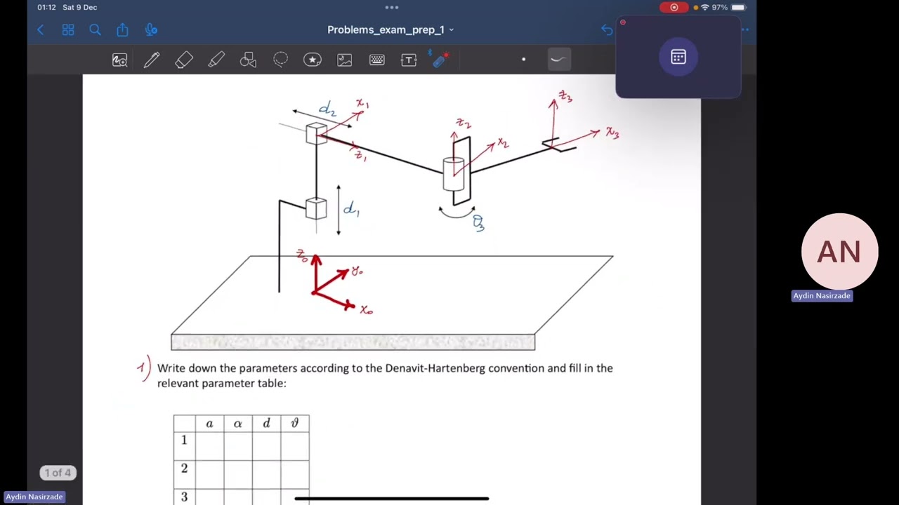
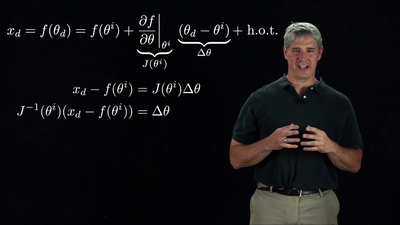
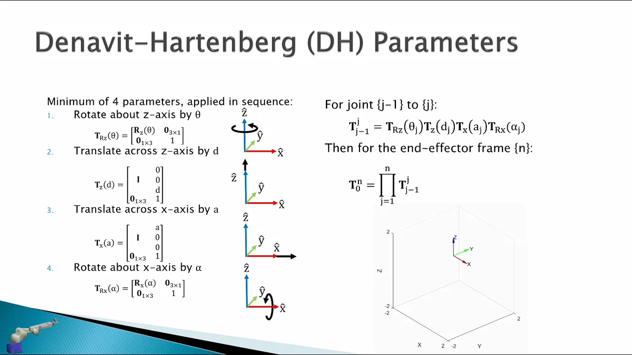
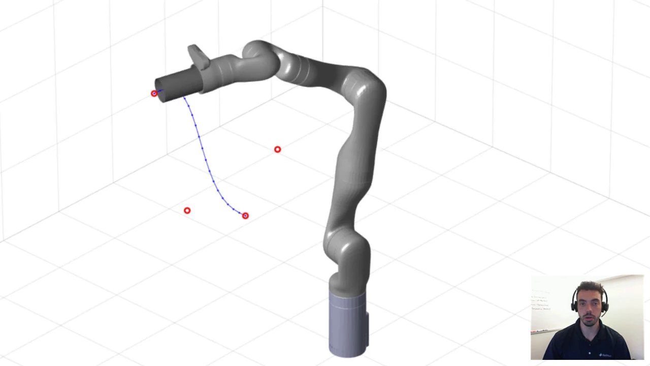
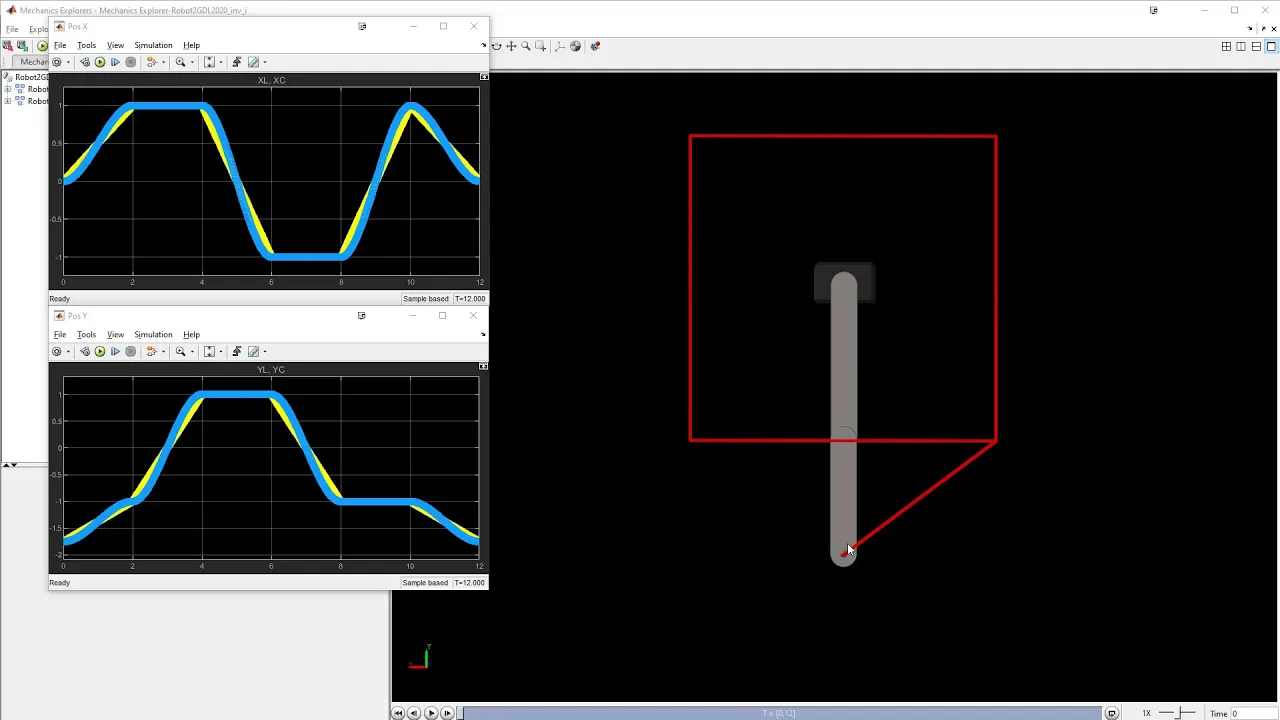
[00:00:00]um hello guys uh today we're going to continue with our inverse kinematics uh study and um what I will do is uh I'm going to do a brief recap on the ik of two degrees of freedom robots and we're also going to look into three degrees of freedom robots and also um uh after this we're we're going to look into basically the kinematics of six axis robots in this course you are not responsible for six axis robots you are only responsible for two or at most three degrees of freedom robots all right um okay so uh regarding last time noticed that we actually had a a small issue when we were doing you know if you do cosine pi/ two right it actually returns a very small number and when you uh basically multiply this by uh or when you uh do some rotations about you know if you do rotations if you apply that basically inside a rotation transformation it will actually return that and uh remember we actually had a problem if I had let's say like a symbolic variable if I actually do you know rotation about Z by Theta and then I do you know rotation about X by pi/ two right and there is an issue here because uh the pi is actually being evaluated as a floating point value or floating Point number and uh this number will actually get multiplied inside this and will actually give us a mess right why because of because of this guy so turned out that we can actually resolve that by evaluating Theta or you know the the value inside the cosine function or or mainly Pi basically if you can actually evaluate that as a symbolic value so what we will do is so you can do simply that rotation about X by Sim of Pi and then divide by two so this will actually solve this problem and now we're good here basically you know this guy will actually be zero and it will not be a very small number that is being carried inside this operation okay uh so uh that is what I wanted to discuss the other thing is let's quickly go back into um you know our discussion last time of the inverse kinematics of two degrees of freedom robot you said the inverse kinematics is what the inverse kinematics is that given a position or given a cartisian position of your end Factor find me the position or the joint positions of the robot and in the case of a two degrees of freedom robot obviously we have t one and two and XE and Y are provided for you the first thing that you want to do is you want to look into this you know virtual lens L and we know L is going to be equal squ root of x e^2 plus y e squ right because you know this is the x coordinate of the end factor and then this is a y coordinate of the end Factor uh then the first thing that I can do is actually I can find t two right before finding t one so I find T 2 and the way I can do that is I can look into this U you know right triangle and I know now l s which I already know is also going to be equal to L1 plus L2 cosine Theta 2 s right plus L2 sin thet 2 square so with that portion right squared if you expand this you will see that you will actually end up with this guy right L1 squ plus L2 squ + 2 L1 L2 cosine Theta 2 and I can actually use that to find th 2 so cosine is equal to this by rearranging this and solving for cosine thet 2 then I can actually find what Theta 2 is by doing the inverse of that and we know basically the inverse the cosine of an angle basically is two solutions right two angles the cosine of two angles will give me the same cosine right so if Theta is like that and Theta is actually like that I will actually get the same value right this is my cosine right and then this is my sign so this so plus Theta and then minus Theta will actually give me the same cosine so Theta 2 is equal plus or minus this guy and whatever solution I actually choose here I will only choose it only once so if I choose the positive value then after we solve for Theta one it will actually apply also on Theta one right so we have cosine or I'm sorry is plus minus that so here for example I Choose You know the minus solution or I could even choose a positive solution okay now let's look into how we can find Theta one so the way we find Theta one is so now we have Theta 2 already uh we can actually find the one by looking into the difference between these two angles beta right beta is the angle that this virtual line makes with the x-axis and then Alpha is the angle that this virtual lines makes with uh with link one and Theta one is nothing but beta minus Alpha right now I've already solved th 2 I can actually find Alpha what is Alpha tangent Alpha is equal to this guy over this guy right opposite over adjacent what is opposite I already have Theta 2 opposite is going to be L2 time sin Theta 2 and the adjacent is going to be L1 plus L2 cosine okay and we said you don't want to use Alpha is equal to inverse tangent of this guy or a tan no you want to use a tan 2 why because a tan2 will actually tell you on which quadrant you are if both of the angles are negative right if both of the values are you know kind of negative uh yep uh okay so if you have a value here and then a value here so basically right so if you are here uh it will actually not know it will think you are here right why because minus over minus is positive so actually return this angle so you have Theta for example and then you can actually have also theta plus pi right sometimes your motor is actually theta plus pi is not here this is a physically different position than th right so if you use a and two you're good right so whatever values you have if both of them are negative it will actually return theta plus pi all right so now we have Alpha what is beta so we can simply find beta uh by this guy right so I know tangent beta is equal to ye over XE right so again beta is equal a 2 y XE right and already have 2 right so I know Alpha now I can find Theta one is going to be equal to let's say you know Alpha minus beta or Alpha minus beta beta is here in this case so uh or minus Alpha so minus minus Alpha right plus beta okay so uh this is it regarding the ik of two degrees of freedom you know uh you know rot uh rotational rotational joints basically or are or two degrees of freedom are are robots uh let's look into the three degrees of sedom case and um and this is what we have let me just close this down a little bit uh so regarding uh three degrees of freedom robots is uh typically it would look like this right if it wasn't mainly like you know if it didn't have any like linear DRS Etc this is what we're going to be dealing with and we will see in the next lecture that uh the combination of this three degrees of freedom robot with a wrist will actually give me the six axis uh robot configuration but let us actually see how we can actually solve what is TAA one Theta 2 and TAA 3 for this uh for this robot and in the case of the inverse kinematics of this robot ex it essentially what are you providing you are providing the X Y and Z of your end of factor so you are basically providing the position of that point and then you are solving for Theta one Theta 2 and theta 3 okay let's put that in you know uh in more context what do we have so this is my Theta one right and then these are you know proper d h frames this is my z0 Z1 and and then Z2 and uh and how can I solve Theta one so here we'll do basic gometry we'll use geometry to be able uh to find uh to find Theta one and th 3 so how is Theta one I know simply that tangent th 1 is equal to YC over XC right so th 1 is equal to a t 2 YC comma XC right now we found that uh Second Step is we need to find Theta 2 and theta 3 if you actually look into this you will see that uh this portion of the robot link two and Link three it it is in a sense like a two degree of Freedom robot that is actually in this Frame right uh okay so I can actually now find Tata three and then find Tata 2 right um but before doing that let me go to the next slide okay this is the definition of 8 and2 uh this is what we did for thata one right 8 and 2 Y and then x c uh we'll start basically by finding that three right based on this guy right and then we said this guy is exactly exactly look like the one that we actually just solved right uh that size a little bit okay here we go um all right so what is T three well I actually have this guy right so what is le initially so I know Le has to be equal to what uh so the coordinate of XC YC and DC is provided to me right I need to know l e so l e is actually nothing but XC s + YZ square plus zc minus L1 squ so basically you are uh kind of transforming this guy into this by uh you know removing the distance L1 right so zc minus L1 will actually give me that distance right and now L is equ nothing but that guy and to solve theta 3 basically I will use exactly what I just did here right so I know l s has to be equal to what L2 S Plus L3 cos or equal to L2 plus L3 cosine theta 3 squ right which is this guy plus L3 sin theta 3 Square so we're good here we got that after you expand this you end up with this guy and you already know l so you can actually solve for cosine theta 3 okay now we solve theta 3 next step is we need to find T 2 how do I find T 2 exactly what we did before we know that t 2 is equ Al to Beta minus Alpha and I already know alpha alpha is going to be equal to 812 this guy over this guy which is L3 sin Theta 3/ L2 plus L3 cosine theta 3 okay final thing is going to be beta uh how do you find beta right which is this guy so you're going to Beta is going to be equal to this height here which is zc minus L one which is all good right divide by this guy so what is this lens right here so this lens from here to here so so here we're actually in the X1 frame we're not along x0 we're along X1 and if you see basically uh beta right so beta is going to be this guy right let me actually throw that okay here we go so it's going to be this guy right which is z of C minus L1 right how about this guy what is the L of this guy this guy is what is nothing but XC s Plus or square root of x c square plus YZ Square y c square right okay let's clear that come back here and then you'll see okay so that's it right so beta is equal to zc minus L1 and square root of x square so if you use this basically now we find Thea 2 so basically simply using geometry we can find the angles of the three degrees of freedom robot that is basically just rotational rotational rotational okay and then we will actually see that we will use this configuration and then we're going to attach a rist to it and then we'll be able to solve theomatics of six axis robots so in this course you are not responsible for the inverse chemtics of this axis robots you just need to be basically you need to understand this very well basically and how we actually do the ik of two and three degrees of freedom robots and now that I actually have soled for my angles I can actually use my homogeneous transformations to be able to plot the robot right so what is h so basically now uh let me just start this okay now that I actually have Theta one Theta 2 Anda 3 I can do my homog Transformations between the various frames I can do h01 is going to be what rotation about Z by Theta one so now your x0 is along X1 then you translate about Z by L1 then you uh about x two right because uh you know after you do this so you about z0 by T you translate now your x0 is along X1 right but your z0 is up so you still need to rotate about x by/ 2 to basically put z0 along Z1 right so that is why you need this last transformation once you are here basically it's nothing but you rotate about Z and then you translate along X right so here we rotate about Z by 2 and then we translate along X by L2 plus one is we rotate about Z by 3 and then we translate about X by3 now that we actually have H1 h12 and then H2 3 we can actually multiply all of these together and then I can actually obtain the position of my Vector based on T so now we have the ik and then the FK so I can literally provide simply x y and then z i can calculate my tatas and then I can actually plot the robot so this will give me a sense of how I can actually animate an industrial robot right so you start with the inverse kinematics inverse kinematics will give you the joint positions then you use the forward kinematics or the H transformations to be able to actually plot the robot in mat laab this is how it actually looks like um you know we basically provide the cartisian point or you know the where is the tool center point for example in this case XC YC zc right I can change those whatever I want to do those you know I can also provide the link lenses on the various robot and then based on these basically I'm actually solving whatever t one uh based exactly on what we just did right T one is provided a and 2 yxc we've already done that L we solve T 3 first and then we actually obtain t two okay and you can here obviously change any you know dimensions in a robot or you can change where you would like your end factor to be and based on that we actually solve all these guys and after we do those obviously like I said we do the homogeneous Transformations and after the transformation we can actually obtain the origins of the various frames and then uh we can plot them right we said last time we can plot the link right based on the line function matab and then we can plot the various points in by doing so basically we can actually plot and then animate the robot and be able to actually visualize how the robot is actually going we can actually uh you know simulate the robot moving along a straight line or you know um X Direction y direction or along any any line basically you would be able to actually simulate that because now you have the inverse kinematics model working all right guys so that is it regarding this lecture in next lecture I will actually go over you know how we can actually attach a a a a a rist to this guy and then you know to be able to control the orientation of the robot right or the orientation of theor this this particular this configuration actually will only solve Theta one 12 three at this point right and I will not be able to actually control how I'm actually you know orienting this Vector right it will simply go to this point but we have no mean of actually doing the orientation if you want to do orientation control you actually have to add three more joints to this and this is called actually the rist any questions on that guys email me and I'd be very happy uh to help you out okay bye-bye